How convolutional neural networks work, in depth
Skills:
Neural Network Basics90%
Key Takeaways
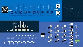
This video teaches how convolutional neural networks work in depth
Full Transcript
when you hear about artificial intelligence about 1/2 of the time what people are talking about is convolutional neural networks understanding how they work is really helpful in getting a peek behind the curtain at the magic of artificial intelligence so we're gonna walk through it in some detail convolutional neural networks takes images and from them they learn the patterns the building blocks that make them up so for instance in the first level of this network you might learn things like line segments that are at different angles and then at subsequent layers those get built into things like faces or element of cars depending on the images that you train the network on you can pair this with reinforcement learning algorithms to get algorithms that play video games learn to play go or even control robots so to dig into how these work we'll start with a very simple example much simpler than all of these a convolutional neural network that can look at a very small image and determine whether it's a picture of an X or an O just two categories so for example this image on the left is an 8 by 8 pixel image of an X we want our network to classify it as an X similarly with the image of the O we want the network to classify it as an O now this is not entirely straightforward because we also wanted to handle cases where these inputs are of different sizes or they're rotated or they're heavier or they're lighter and every time we'd like it to give us the correct answer a human has no problem looking at these in deciding what to do but for a computer this is much harder when trying to decide if these two things are equal what it does is it goes through pixel by pixel black pixels might be a minus 1 white pixels might be a plus 1 and it'll compare them pixel by pixel find the ones that match and here the red pixels are the ones that don't match so a computer looking at this would say no these are not the same they have some matches but they have a lot that don't match so the way convolutional neural networks do this one of the tricks they use is that they match pieces of the image so you can look at these pieces and shift them around a little bit but as long as the tiny bits still match then the overall image is still considered a pretty good match so these tiny bits might look like this we'll call them features you can see the one on the left looks like a diagonal arm of the X that's leaning left the one in the middle looks like the center of the X where it crosses and the one on the right looks like a diagonal arm leaning right and you can see how these different pieces these different features of the image match different patches within the overall image so the math behind finding this match applying features is called filtering it's pretty straightforward but it's worth walking through the way that is done is you align the feature up on the image patch you're concerned with multiply pixel by pixel add up the values and then divide by the total number of pixels this is one way to do it here for instance we start with this feature of the arm of the X leaning left we align it with this arm on the image and we start with the upper left pixel and we multiply both values one by one equals one now because we started with the upper left pixel we can keep track of our answers here so this pixel when multiplied equals one the upper center pixel is minus one in both the the feature and the image so minus 1 times minus 1 is also equal to 1 so that when you multiply them and you get a 1 that indicates a perfect and a strong match and we can continue doing this throughout the entire feature and the entire image patch and because they are a perfect match every single one of these matches will come back as a one and so to find the overall match we just add up all these nine ones divided by the total number which is nine and we get a match of one now we can create another array to keep track of how well the feature when placed in this position match our image so this average values one will put a 1 right there to keep track of that you can see what it looks like if we were to move this feature then and align it to a different patch so let's say we move it down to the center of the X and we go pixel by pixel and find what matches and after a few pixels we actually find one that doesn't match we end up with a minus one times a plus one giving us a minus one back this indicates a non match of these pixels and as we go through the rest of the feature we can see that there are a couple pixels that don't match so here when we add these up and divide by nine we get a number that's less than one point five five so that indicates a partial match but not a perfect one it turns out you can go through and do this for every possible location in the image you can chop it up into every possible image patch compare the feature to each one and here's what you would get in this particular case this is what convolution is it's taking a feature and applying it across every possible patch across a whole image and you can see here why it's called filtering what we have is a map of where this feature matches the image you can see a strong bunch of plus ones on the diagonal line from the lower right to the upper left and then lesser values everywhere else so it's a filtered version of the original image that shows where the feature matches you can do this we can represent this with this notation we just invented this little convolution Oppel operator for shorthand and we can do this with our other features as well we can see where our Center X matches not surprisingly it matches strongest in the center of the image we can see where our leaning right arm matches and not surprisingly it matches along this diagonal from the lower left to the upper right we have 3 filtered versions of the original image so this is what a convolution layer in a convolutional neural network does it has a set of features in it and it can be 3 or 30 or 300 or 3000 but it has a set of features and it takes the original image and returns a set of filtered images one for each of the features so this is how we'll represent it that's the number one ingredient in convolutional neural networks that is the magic special sauce the special trick that gets from a non exact match and let's the algorithm is able to pull out ok well it's not a perfect match but it's still a pretty good match because it does this convolution and moves the feature across the image and finds everywhere that it might match another piece of this is called pooling so we took our original image and now we have a stack of images what this step does is it shrinks it down a little bit we start by picking a window size usually 2 or 3 pixels picking a stride usually 2 pixels has been shown to work well and then walking this window across the filtered images and then from each window taking the maximum value that you see so this is called max pooling so to see how this work so we start with one of our filtered images we have our window which is two pixels by two pixels and within that the maximum value is one so we create another little array to keep track of all of our results and we put a 1 in it and then we step it over it by our stride which is 2 pixels look at the window choose the maximum value in this case it's 0.33 record it and go again and we keep doing this recording the maximum value each time all the way through the image and when we're done we have which if you squint looks like a shrunken version of the original we still have this strong set of plus ones on the diagonal from upper left to lower right and then everywhere else it's less than that so it maintains kind of the original signal but shrinks it down kind of picks off the high points and this gives us a smaller image but still similar to the original and we can just represent it with this little shrinking arrow we can do this with each of our filtered images and again you see that very roughly the pattern of the original is maintained so in a pooling layer a stack of images becomes a stack of smaller images now the last ingredient we need is normalization so this keeps the math from breaking by taking and tweaking these values just a little bit it takes everything that's negative and changes it to zero this keeps things from becoming unmanageably large as you progress through subsequent layers this function is called a rectified linear unit it's a fancy name for something that just takes anything that is negative and makes it zero so a point seven seven not negative it doesn't touch it but a minus point one one it's negative just bumps it up to zero and by the time you've gone through all of your images and done this all of your pixels and done this this is what you have so everything that was negative is now zero so just a nice little bit of normalization some conditioning to keep things numerically well-behaved so a stack of images becomes a stack of images with no negative values now you can notice that the output of one layer looks like the input to the next there are always arrays of numbers an image and an array of number are the same thing they're interchangeable so you can take the output of a convolution layer feed it through the rectified linear units a feed that through the pooling layer and when you're done you have something that has had all of these operations done to it and in fact you can do this again and again and this recipe can imagine making like a scooby-doo sandwich of all of these different layers again and again and in different orders and some of the most successful convolutional neural networks are kind of like accidentally discovered groups of these that just happen to work really well so they get used again and again so over time each convolution layer filters through a number of features each rectified linear unit changes everything to be non-negative and each pooling layer shrinks it so by the time you're done you get a very tall stack of filtered images with no negative values that has been shrunken down in size now by the time we've gone through several iterations of this we take and run it through a fully connected layer this is more of a standard neural network where every input gets connected to everything in the next layer with a weight every single value you can think of it as a voting process so every single pixel value that's left in these filters shrunken images gets a vote on what the answer should be and this vote depends on how strongly it is tends to predict an X or an O when this pixel is high is this output usually an X or is it usually an O so you can see for this particular input the input was an X here's what the imaginary convolve din filtered values are and over time we would learn that these things that are high when it sees an X get a strong vote for the X category similarly if you have an input that's an O these final pixel values that tend to be really high when the right answer is RO is o gives a strong vote for the O category the thicknesses of these lines represent the weights the strength of the vote between these pixels and these answers so now if we get a new input that we've never seen before these might be the final pixel values we can use these votes and do a weighted voting process for both of these add them up and in this case you know it's a point 9 to total for X and a point 5 1 total for 0.92 is obviously more than point 5 1 we declare X the winner so this input will have been categorized as an X so this is a fully connected layer so it just takes a list of feature values in this case are filtered shrunken pixels and it becomes a list of votes for each of our output categories in this case an X or an O now these can also be stacked you can have like little they call them hidden layers but like secret hidden categories in between here so one votes on the first layer votes on the first set of hidden categories and then those vote on the next layer and so forth until you get to your final ones well dig into this more in just a little sec but these are all stack on to the end now to go into the next level of detail on these neural networks set aside are X and O detector for a while there we had 8 by 8 pixel images so 64 pixels in all consider now a 2 by 2 pixel image so just a 4 Soul camera and what we would like to do is categorize the images that it takes as either being a solid image all light or all dark a vertical image a diagonal image or a horizontal image now the trick here is that simple rules can't do it so both of these are horizontal images but the pixel values are completely opposite in both of them so you can't say well if the upper-left pixel is white and the upper right pixel is white then it must be horizontal because that's violated by the other one now of course you could do more complicated rules to do this the point is that when you go to larger images you can't make simple rules that capture all the cases that you want so how do we go about it we can take these four input pixels and break them out we call them input neurons but they just take these pixels and turn them into a list of numbers the numbers correspond to the brightness - one is black plus one is white zero is middle gray and everything else is in between so this takes this little image and turns it into a list of numbers that's our input vector now each of these you can think of it as having a receptive field this is an image which makes the value of this input as high as possible so if you look at our very top input neuron the image that makes that number as high as possible is an upper left pixel that's white that makes the value of that one and it doesn't care what the other pixels are that's why they're checkered so you can see that each of these has its own corresponding receptive field the image that makes the value as high as it can go now we're going to build a neuron so when people talk about artificial neural networks and a neuron we are going to build it bit by bit the first thing you do to build a neuron is you take all of these inputs you add them up so in this case this is what we'd get so the neuron value at this point is 0.5 now the next thing we do is we add a weight we mentioned the weighted voting process before so what that looks like is each of these inputs gets assigned a weight between plus and minus one and it gets the value gets multiplied by that weight before it gets added so now we have a weighted sum of these input neurons and we will represent this visually by showing positive weights in white negative weights in black and the thickness of the line being approximately proportional to the weight and when the weight is zero we'll leave it out to minimize visual clutter so now we have a weighted sum of the inputs the next thing that we need to do is squash the result so because we're going to do this a lot of times it's nice if we always guarantee the answer is between plus and minus one after each step that keeps it from growing numerically large a very convenient function is this s-shaped so sigmoid squashing function this particular one is called the hyperbolic tangent there is confusingly something else that's called the sigmoid and it's a little bit different but the same general shape but the characteristic of this is that you can put in your input you know draw a vertical line see where it crosses the curve track that over to the using a horizontal line to the y-axis and you can see what the smashed version the squashed version of your number is so in this case point five comes out to be just under point five point six five comes out to be about point six and as you go up this curve you can see that no matter how large your number gets what you get out will never be greater than one and similarly it'll never be less than minus one so it takes this infinitely long number line and squashes it so that it all falls between plus and minus one so we apply this function to the output of our weighted sum and then we get our final answer so this weighted sum and squash is almost always what people are talking about when they talk an artificial neuron now we don't have to do this just once we can do it as many times as we want with different weights and this collection of weighted sum and squash neurons is you can think of it as a layer loosely inspired by the biological layers of neurons in the human cortex so each of these has a different set of weights here to keep our picture really simple we'll assume these weights are either +1 white lines minus 1 black lines or 0 missing entirely so in this case now we have our layer of neurons we can see that the receptive fields have gotten more complex if you look at the neuron in the first layer on the top you can see how it combines the inputs from the upper-left pixel on the lower left pixel both of the weights are positive those lines are white and so what comes out its receptive field is if both of those pixels on the Left are white then it has the highest value can possibly have if we look at that layer of neurons and look at the one on the bottom we can see that it takes its inputs from both of the pixels on the left I started on the right but it has a negative weight collecting connecting it to the lower right neuron so it's receptive field it's what maximally activates it is a white pixel in the upper right and a black pixel in the lower right now we can repeat this because the outputs of those that first layer of neurons looks a whole lot like our input layer still a list of numbers between minus 1 and 1 and so we can add additional layers and we can do this as many times as we want each time each neuron in one layer is connected to each neuron and the other layer by some weight so in this case you can see how the receptive fields might get still more complex and now we're starting to see patterns that look like the thing that were interested in solids verticals diagonals horizontals by combining these elements now there's one more thing that we can do remember our rectified linear unit we can have different neurons here and instead of a weighted summon squash we can just have something that takes the input and spits out zero if it's negative and the original value if it's positive and so for instance if we have if we have an input whose receptive field is the one on the very top and the second layer all solid white and we connect it with a positive weight to the rectified linear unit near on on top then of course what would maximize that is all solid white input but if we look at the neuron just below that that's connected to it with a negative weight then that that flips everything around and what maximally activates that is an input that's all solid black now we're really starting to get the set of patterns that we can imagine using to decide what are images so we connect these again to a final output layer this output layer is the list of all the possible answers that we expect to get out of our classifier originally it was X's and O's now it's four categories solid vertical diagonal and horizontal and each of these inputs into them have a vote but you can see that very few of them are connected this network assumes that most of those votes are zero so to see how this plays out let's say we start with an input that looks like the one on the left with this is obviously a horizontal image with a dark bar on top and a white bar on the bottom we propagate that to the input layer and then we propagate that to the first hidden layer and you can see for instance the neuron on the very top it combines two input neurons that one is light and one is dark so you can imagine it's summing a plus 1 and a minus 1 and getting a sum of zero so that's why it's gray its value is zero now if you look at the neuron in the very bottom in that first hidden layer you can see that it sums also an input that is negative and one that's positive but it's connected to one by a negative weight and the other by a positive weight so it actually what it sees it's weighted sum is minus 1 and minus 1 so what it is getting you can see is the opposite of its receptive field so that means it's maximally activated but negatively so that's why it's black we move to the next layer and you can trace these things through so anything zero plus zero is gonna get you zero if you look at the neuron on the very bottom of the second hidden layer you can see if it yes it's adding up a negative and a negative both connected by positive weight so it's also going to be negative which makes sense because you can see that it's receptive field is the exact opposite of what the input is right now so it's maximally activated just negative and then when we track this to our next layer you can see that following that bottom pair of neurons because it's a negative value because through the rectified linear unit and becomes 0 so that's gray but if you look at the very bottom neuron there it has it's connected with a negative weight so it becomes positive so that rectified linear unit really likes it so it gives it a maximum value so everything is 0 except for that neuron on the bottom and then finally what that means is that the only output that is nonzero is this horizontal one so this network would classify the input image as being rasaan hole because of this now there's some magic here where did we get those weights where did we get the filters in between this is where we start to get down to the when we talk about learning adaptation you know the learning and machine learning it is all about optimization these are learned through a bunch of examples over time so we're gonna set that aside for just a minute we'll come back to how those get learned but we need to talk about optimization first so consider drinking tea there is a temperature range where it is a delightful experience it's warm and delicious and comfortable if your tea is too much hotter than that it's very painful and not good not fun at all and if your tea is cooler than that its lukewarm and its really mad it's really not worth your time so this area at the top is the pink this is the best this is what we're trying to find in optimization we're just trying to find the best experience the best performance now if we want to find that mathematically the first thing we do is we flip it upside down just because this is how optimization problems are formulated but it's the same type of thing instead of maximizing tea drinking pleasure we want to minimize tea drinking suffering we want to find the bottom of that Valley the lowest possible suffering there's a few different ways we could do this the first is to look at every point on this curve and just pick the lowest one now the trick with that is we don't actually know what this curve is beforehand so in order to pick the lowest one we have to do exhaustive search which in this case would be make a cup of tea have someone drink it ask them how they liked it make another one ask them how they liked that one do it again and again for every possible temperature and then pick the one with the lowest suffering the most enjoyment this is effective very effective also it can be very time-consuming for a lot of problems and so we search for a shortcut now because this is a valley we can use our physical intuition say hey well what if we just had a marble and we let it roll to the bottom of this valley we wouldn't have to explore every single piece of it so this is what's behind gradient descent the way it works is we start not knowing anything about this function we make a cup of tea someone tells us how they like it and then we change the temperature a little bit we make another cup of tea just a little bit cooler we ask someone how they like that and we find out they actually like it just a little bit less that tells us what direction we need to go we need to make our next cup of tea warmer and the change the difference between how much they like those two tells us the slope tells us the steepness gives us the sense of how much warmer we can expect to make that next cup of tea so we make another one and we repeat the process and then we again scoot a little ways off to the side make another cup of tea and figure out again which direction we need to go are we do we need to go warmer to make a better cup or cooler to make a better cup and we repeat this until we get to the bottom of the curve you'll know you're at the bottom when you change the temperature just a little bit and the tea drinker says yeah that's exactly the same I like that just as much as the last one that means that you're there kind of at the flat bottom of the valley so gradient descent is the first level trick for brewing fewer cups of tea there's another thing you can do which is to use curvature this is kind of an advanced method is you can make your original cup of tea and then make one a little bit warmer and one a little bit cooler and you can look to see how that curve of your function goes and if it's very steep and steeper than you know you can take a giant step because you're probably not anywhere close to the bottom and then you can do it again and if that curvature is starting to bottom out then you can take a smaller step because you the signal that you're getting closer to the bottom and it helps you to do this in fewer steps as long as your curve is relatively well-behaved which is not always the case so ways that this can break imagine we're doing this a hot day and actually it turns out that if we were to cool our tee way down we'd get a really nice iced tea which turns out to be even more popular with our tea drinkers but gradient descent would never find this gradient descent always rolls down to the bottom of the nearest valley it doesn't hop around to see if there are any valleys hiding anywhere else another problem is let's say there's a wiggle on our curve there's something happening in the environment we have noisy buses driving by and it affects how people enjoy their tea we might not be able to find this very lowest dip because we might get stuck in a dip further up the curve similarly if we ask our tea drinkers to rate their tea drinking experience on a scale from 1 to 10 we get these discrete jumps in our function and if you imagine a marble rolling downhill it down stairs it doesn't always work well and it can get stuck on a step without making it all the way to the bottom now all of these things happen in real machine learning problems another one imagine you have really picky tea drinkers and if the tea is anything but perfect they hate it hate it hate it and so you have these plateaus on either side and there's no signal to tell you that if you move in a little bit you'll find that deep valley so for cases like this there of course we can always fall back to exhaustive exploration it will the best answer in every single one of those cases but a lot of times we just don't have the time like if I have to brew and measure the pleasure drinking pleasure of 10 million cups of tea to get a good answer to this it's not going to happen in my lifetime so luckily there are some things in the middle that are more sample efficient an exhaustive exploration but a little bit more robust than gradient descent things like genetic algorithms simulated annealing things that they're defining characteristic is they have a little bit of random jumping around they're a little bit of unpredictability and so they make it harder to slip things by them they all have their strengths and weaknesses there tend to be good for different types of problems or different types of pathologies in your loss function but all of them help avoid getting stuck in the local minima the little small valleys that gradient descent will get stuck in they get away with this by making fewer assumptions and they can take a little longer to compute the gradient descent but not nearly so long as exhaustive exploration you can think of gradient descent as being like a Formula One racecar and if you have a really nice well-behaved track it is fast but if you put a speed bump in the track you're done genetic algorithms simulated annealing evolutionary algorithms those are like you know four-wheel drive pickup truck you can take a fairly rough road with those and get where you're going you won't get there in record time perhaps but you'll get there and then exhaustive exploration is like traveling on foot there is nothing that will stop you from getting anywhere you can travel little or literally anywhere but it just might take you a really really long time so to illustrate how this works imagine we have a model that we would like to optimize we have a research question how many M&Ms are in a bag of M&Ms so answering this is easy by you eat it 53 you can count those M&Ms so great we know how many were in the first bag now when I did this I made a mistake and I bought another bag and I tried that one and I got a different answer so now I can answer 53 or I can answer 57 either way I'm only right half the time because I can't capture both bags with one answer and I could answer somewhere in the middle but that's never right I have never opened a bag that had 55 M&Ms in it so it's unclear that that's the right answer either and the situation does not improve with the more bags of M&Ms that I ate it just gets a little bit out of control and so I changed my goal from answering the answer answering the question right to answering the question in a way that is less wrong so in order to do that I have to get really specific about what I mean by how wrong I am and to do that I have this distance function this deviation which is the difference between my actual guess and the actual number of M&Ms in a bag so we call for for bag number I this deviation is D sub I it's just the difference between the guess and the actual number and then I have to take this deviation and turn it into a cost so one common way to do this is to square it it's a nice as the further away things get kind of the more costly it is perceived as and it goes up faster so if there's a bag that's off by twice as much as another the cost is four times so I really it penalizes the things that are way off the things that are close it doesn't penalize so much and if we don't care if we don't want to overly penalize the things that are way out there we could use the absolute value of the deviation so if it's off by twice as much just be twice the cost but really we could use anything we could use the square root of the absolute value we could use ten to the power of the absolute value of this deviation anything that goes up the further away you get from zero we'll stick with squared deviation this is super common it has some nice properties and makes for a good example so for the total cost of any guess that we make if I guess an estimated bags M&Ms in a bag then the loss function is fancy curlicue L of that guess is just adding up the square of the deviation associated with each bag of M&Ms d1 through DM squared so each deviation is actually the number of M&Ms in that bag - the guess so I square that and we can write that with fancy summation notation like this so this is my loss function this is the total cost this is how wrong I am when I make a guess and esthe so because we have computers you can write a little bit of code and you can do exhaustive exploration and I can say if I guess anything between 40 and 70 how wrong would I be with this data and you can plot it and visually we can look at this and we can say hey look there's the lowest value and we can say what is the value of the guess that gives me the lowest loss that's what that argument that notation means right there and this best guess is just about fifty five and a half M&Ms problem solved so this is an example of numerical optimization where we calculate this loss function and then we can do essentially because it simulated we can do exhaustive exploration and just pick off the lowest value now for this particular example there's a fun other way to find it we know at the bottom of this curve the slope is zero it's the only place in the whole curve where that's true where it's flat we can use a little bit of calculus to find that feel free to tune out if calculus is not your thing but it's not too bad so we find the slope of the loss function with respect to our guesses and we set it equal to zero and we solve it to find what for what guess is that true so we take our loss function this sum of the square of the differences of the count and the guess and we take the derivative of that with respect to our guests and the derivative of a sum is the same as the sum of the derivatives we take the derivative of that just bring down the exponent so two times that summed because all that's equal to zero we can divide it by two and it'll still be true so now the sum of our deviations is zero so to further simplify this it's the sum of all of the counts of the actual bags times the sum of our guess once for each bag if we have m bags then it's M times our guests and then we can move that to the other side of the equals sign and divide both sides by the number of bags M and what we get is that our best guess is the sum total of the number of M&Ms we found in all the bags divided by the number of bags or the average count per bag so this is a really slick result and it's things like this they make people so excited about optimization a little bit of math and calculus you can get this nice theoretical result now it's worth noting that this is only true if you use a deviation squared as your cost function so that's one reason people like it so much is because it tends to give some nice results like this but there is this analytical shortcut to find what the best guess is we're going to come back to this in a few minutes now how does optimization change how do we use it in our neural network to find these weights and these features so what we want to do we know what our error function is its how wrong our guesses are so in this case we have a labelled data set which means that a human has already looked at this input on the left and I said hey that's a horizontal image the truth values are what we know should be the right answer zero votes for everything except horizontal that should have a vote of one so let's say initially we've got a neural network that all the weights are random and it gives us nonsense results it says well yeah everything is has some number associated with it but it's nothing like the right answer well we can find the error for each category and add it up and find a total error and this is how wrong our neural network would be for this one example here is our loss here's our error now the idea with gradient descent is we're not just adjusting one thing we're not just adjusting our guess of the number of M&Ms we're adjusting many things we want to go through and adjust every single weight in every single layer to bring this error down a little bit now that is a little bit challenging to do because in order to do that one thing you can do is find a analytical solution like we did before to go through and move our guess a little bit up and a little bit down and find the slope is really expensive when you consider that this is not a one-dimensional problem anymore it might have hundreds or millions of different weights that we need to adjust so calculating that gradient that slope requires hundreds or millions of passes through the neural network to find out which direction is downhill enter back propagation so remember we found the nice analytical solution to what we had going on in the case of the mm estimate so what we would love to be able to do something like that again if we had an analytical solution we could jump right to the right answer so slope in this case it's change in weight our sorry it's change in error for a given change in weight that's the slope here so there's lots of ways to write that but Delta error Delta weight D air d weight will use this partial error partial weight just cuz it's most correct but all these things mean the same thing if I change the weight by 1 how much will the error change what is the slope so in this case it would be minus 2 and we would know that we need to increase the weight in order to get closer to the bottom this tells us not only the direction we need to move but gives us a sense of about how far we should go doesn't tell us exactly where the bottom is but it tells us which way it needs to adjust now if we do know the error function example we can make a an analytic solution and we can find that we can calculate that slope exactly so in this case the change in error for a given change in weight is just the derivative of our error function here which is in this case is the weight squared so the derivative is 2 times the weight the weight is minus 1 and so the answer is a slope of minus 2 that tells us what we need to know about which way to adjust now with neural networks of course they're a lot more complex than that but we can actually analytically compute the slope of the function where we are we don't know where the minimum is but we can find the slope without having to recalculate the value of everything each time and this is how it works imagine the world's most trivial neural network that has one input one output one hidden layer with one neuron in it so it's got an input connected by a weight w1 to an intermediate value connected by a weight W to to an output value so the intermediate value is just x times that weight so the derivative of Y with respect to the weight is X what that means is if I change w1 and I move it by 1 then the value of Y will change by the value X whatever X is we have the slope of this piece of the function similarly it's straightforward we can just read off that whatever the value of y is multiplied it by the way W 2 we get e so if we want to find the slope of the error function for a given change in Y the answer is w-2 if I changed Y by 1 unit then the error changes by the amount w2 now chaining means that we can take these two things and just multiply them together so by inspection we can see that in this little neural network if we take X multiply it by w1 multiply that by w2 we get the error e now what we'd like to know is if I change that w1 by a certain amount how much does the error change in this case we just take that whole expression and take the derivative with respect to w1 and fairly trivial bit of calculus it comes out to be x times w2 and what we can see then is we can substitute in these steps this change in y with respect to w1 is same as xw2 is the same as the change in error with respect to Y and what this breaks down is if we want to step down the chain we want to know how much a change in w1 affects the error what is de dw1 we can actually break it down into steps and say okay well if I change w1 how much does y change and then if I change Y how much does the error change this is chaining and this is what lets us if we know which way we want to change the error it lets us calculate how much we can change this weight to help that happen and there's nothing to prevent us from doing this again and again if I have a weight that's deep into my neural network and I want to know how much my error is going to change if I tweak it up or down I want to know the slope of my loss function with respect to that weight then I can just break it down and say okay well if I change the weight how much does a change if I change a how much does B change I change B how much does C change and chain it all the way down now it's called back propagation because in order to calculate it we actually need the value at the end we have to start with the error value didn't a in order to calculate each of these all the way back down into the depths of the network but still we can do that now the way the reason you have to go backwards is that let's say we want to know what this should be if I change the error if I change a how much does the error change like well let's assume that I already know how much the error is gonna change if I change B what is this back propagation step what is the additional link I need to add to this chain it's like well it's how much does B change if I change a if they're connected by a weight then how do I incorporate that weight we know that tuner connected in this way are represented by this B is the weight times the value of a and so we can just take a little derivative here and get the change in B with respect to a is w so this step in the back propagation change can be represented by whatever that weight is cool now we know that we have sums in our neural network that's another thing we have to handle if I know how much my error changes with a change in Z then how much would it change with a change in one of the inputs to this to Z where that input goes into a sum well I have can write the expression for Z adding up all the inputs if I want to know how much Z changes with respect to a change in a I just take the derivative and it is turns out to be 1 so this is a trivial back propagation step now the most interesting one of all if I know how much the error changes with respect to a change in B and then I want to know how much it changes with the input and to that sigmoid function then I can just say ok well a sigmoid function mathematically looks like this and I can take the derivative of B with respect to a and one of the beautiful things about the sigmoid function is that the derivative actually looks like this it's just the value of the function times 1 minus the value of the function which is one of the reasons that sigmoids perhaps are so popular in deep neural networks so this step is also straightforward to calculate in none of these steps have we had to recalculate all of the values in the neural network we've been able to rely on things that have already been calculated what the values are at each of these neurons that's what makes backpropagation so mathematically efficient and that's what allows us to efficiently train neural networks that is why each element in a neural network no matter how exotic it is needs to remain differentiable so that we can go through this exercise of finding what the link in the chain is when we're doing the chain rule on our derivatives so that we can compute the back propagation we can back propagated and again rectified linear units if we know how much the output affects a change in error we want to know how that extends to the input we can write the function of a rectified linear unit we can take the derivative of it and then use that in our chain rule so imagine now that we have this labeled example we calculate the answer that this random neural network that's not special at all it'll give an answer that's completely wrong and then we back propagate the error and adjust every one of those weights a little bit in the right direction and we do that again and again after you do that a few thousand times this stochastic gradient descent goes from this fully connected totally random neural network to something that is a lot more efficient and that is able to give answers that are much closer to the right answer so coming back up to our convolutional neural networks these are the fully connected layers that's how they're trained they can also be stacked this back propagation applies not only to these fully connected layers but also to the convolutional layers and the pooling layers we won't go through and calculate the chain rule for them but you can do that as well and going through this this whole stack of different layers gets trained on a bunch of examples in this cases of labeled X's and O's give it a bunch of inputs that we know the right answer to and we let it adjust all of those connections not only that it also adjusts all of the pixels in the features for each convolutional layer so it learns not only the weights but also the features and then over time those representations become something that lets it predict very well what is an X and what is an O on top of that there are other things that we can use optimization for so that there's a bunch of decisions here that we haven't addressed yet how do we know how many features to put in each convolutional layer how do we know how big those should be how many pixels on the side how do we choose the size and stride of our pooling windows in our fully connected layers how many layers do we have and how many hidden neurons do we put in each each of these decisions are called hyper parameters they are also values that we get to choose but they're the next level up they kind of control how everything happens below and in order to see how well they perform we have to train the whole thing on all the images start to finish so but the same principles apply we can adjust these and choose them to get the best result possible in a lot of cases it's worth pointing out that there's just not enough computation available in the world to try out all the possible examples and so what we have right now are some recipes some things that researchers have stumbled on to that seem to work well and they get reused but there are a lot of places a lot of combinations of these hyper parameters that actually haven't been tried yet and so there is always the possibility that there are some combinations that work even much better than what we've seen so far now we don't have to use convolutional neural networks for just images any two-dimensional or three-dimensional data works well the thing that matters is that in this data things that are closer together are more closely related than things far away it matters if two things are an adjacent rose or an adjacent columns so in images this is plainly the case the location of a pixel in an array of pixels is part of the information if you were to randomly jumble the rows and columns that would lose the information that's there that's what makes this well suited to convolutional neural networks anything you can make look like an image may also be suited to convolutional neural networks for instance if you're working with audio you have a really nice x-axis your columns can be subsequent time steps you don't want to jumble those because the time the order in which things are current time matters and you can make your rows the intensity in different frequency bands going from low frequency to high frequency again the order matters there and so being able to take sound then and make it look like an image you can apply this processing to it and find patterns in the sound that you wouldn't been able to find conveniently any other way you can also do this with text with a little bit of work you can make each of your rows a different word in the dictionary and then you can make your columns the position and sentence or a position location that it occurs in time now there are some limitations here convolutional neural networks only capture local spatial patterns so if your data can't be made to look like an image or if it doesn't make sense to then they're less useful so for example imagine you have customer data that has columns representing things like names and ages addresses emails purchase transactions browsing histories and these customers are listed if you were to rearrange the rows or rearrange the columns the information itself wouldn't really be compromised it would all still be there it would also be queryable searchable and interpretable convolutional neural networks don't help here they look for spatial patterns so if the spatial organization of your data is not important it will not be able to find what matters so rule of thumb if your data is just as useful after swapping your columns with each other then you can't use convolutional neural networks you shouldn't use convolutional neural networks that's a big takeaway from this so they're really good at finding patterns and using them to classify images that is what is they are the best at now the takeaway from this is not that you should go and code up your own convolutional neural networks from scratch you can it's a great exercise it's a lot of fun but when you go to actually use it there are a lot of mature tools out there that are helpful and just waiting to be applied to this the takeaway from this is that you will be asked to make a lot of subtle decisions about how to prepare your data and feed it in how to interpret the results and how to choose these hyper parameters for this it helps to know what's going to be done with your data and what it all means so that you can get the most out of these tools all right good luck
Original Description
Part of the End-to-End Machine Learning School Course 193, How Neural Networks Work at https://e2eml.school/193
slides: https://docs.google.com/presentation/d/1R-DnrghbU36jO8X4scbrrlx6gFyJHgSL3bD274sutng/edit?usp=sharing
machine learning blog: https://brohrer.github.io/blog.html
Watch on YouTube ↗
(saves to browser)
Sign in to unlock AI tutor explanation · ⚡30
Playlist
Uploads from Brandon Rohrer · Brandon Rohrer · 37 of 60
1
 2
2
 3
3
 4
4
 5
5
 6
6
 7
7
 8
8
 9
9
 10
10
 11
11
 12
12
 13
13
 14
14
 15
15
 16
16
 17
17
 18
18
 19
19
 20
20
 21
21
 22
22
 23
23
 24
24
 25
25
 26
26
 27
27
 28
28
 29
29
 30
30
 31
31
 32
32
 33
33
 34
34
 35
35
 36
36
 ▶
▶
 38
38
 39
39
 40
40
 41
41
 42
42
 43
43
 44
44
 45
45
 46
46
 47
47
 48
48
 49
49
 50
50
 51
51
 52
52
 53
53
 54
54
 55
55
 56
56
 57
57
 58
58
 59
59
 60
60

Robot Learning with a Biologically-Inspired Brain (BECCA)
Brandon Rohrer
BECCA talk at AGI 2011
Brandon Rohrer
Robot Learning with a Biologically-Inspired Brain (BECCA), The Sequel
Brandon Rohrer
BECCA listens to The Hobbit
Brandon Rohrer
Learning the building blocks of speech: BECCA extracts a hierarchy of audio features
Brandon Rohrer
BECCA listens for sound effects in The Hobbit
Brandon Rohrer
BECCA finds movie trailers while watching the Big Bang Theory
Brandon Rohrer
Listening for unexpected sounds: BECCA detects anomalies in audio data
Brandon Rohrer
Learning the building blocks of vision: BECCA extracts a spatio-temporal hierarchy of features
Brandon Rohrer
Watching for the unexpected: BECCA detects anomalies in video data
Brandon Rohrer
BECCA finds a stationary target
Brandon Rohrer
BECCA finds a stationary target at 3X speed
Brandon Rohrer
BECCA watches the X-men and Bruce Lee
Brandon Rohrer
BECCA plays Quidditch
Brandon Rohrer
BECCA chases a ball
Brandon Rohrer
BECCA chases a ball, part 2
Brandon Rohrer
Becca chases a ball, part 3
Brandon Rohrer
BECCA creates features from MNIST
Brandon Rohrer
How reinforcement learning works in Becca 7
Brandon Rohrer
Deep Learning Demystified
Brandon Rohrer
How Data Science Works
Brandon Rohrer
How Convolutional Neural Networks work
Brandon Rohrer
How Bayes Theorem works
Brandon Rohrer
How Deep Neural Networks Work
Brandon Rohrer
Recurrent Neural Networks (RNN) and Long Short-Term Memory (LSTM)
Brandon Rohrer
How Support Vector Machines work / How to open a black box
Brandon Rohrer
How autocorrelation works
Brandon Rohrer
Getting closer to human intelligence through robotics
Brandon Rohrer
A minimalist's guide to slicing and indexing pandas DataFrames
Brandon Rohrer
How decision trees work
Brandon Rohrer
Data scientist archetypes
Brandon Rohrer
How to use python's datetime package
Brandon Rohrer
How optimization for machine learning works, part 1
Brandon Rohrer
How optimization for machine learning works, part 2
Brandon Rohrer
How optimization for machine learning works, part 3
Brandon Rohrer
How optimization for machine learning works, part 4
Brandon Rohrer
How convolutional neural networks work, in depth
Brandon Rohrer
How to pick a machine learning model 4: Splitting the data
Brandon Rohrer
How to pick a machine learning model 3: Choosing a loss function
Brandon Rohrer
How to pick a machine learning model 2: Separating signal from noise
Brandon Rohrer
How to pick a machine learning model 1: Choosing between models
Brandon Rohrer
How to pick a machine learning model 5: Navigating assumptions
Brandon Rohrer
What do neural networks learn?
Brandon Rohrer
Interview with iRobot's Director of Data Science Angela Bassa
Brandon Rohrer
How Backpropagation Works
Brandon Rohrer
Evolutionary Powell's method: A discrete optimizer for hyperparameter optimization
Brandon Rohrer
1D convolution for neural networks, part 1: Sliding dot product
Brandon Rohrer
1D convolution for neural networks, part 2: Convolution copies the kernel
Brandon Rohrer
1D convolution for neural networks, part 3: Sliding dot product equations longhand
Brandon Rohrer
1D convolution for neural networks, part 4: Convolution equation
Brandon Rohrer
1D convolution for neural networks, part 5: Backpropagation
Brandon Rohrer
1D convolution for neural networks, part 6: Input gradient
Brandon Rohrer
1D convolution for neural networks, part 7: Weight gradient
Brandon Rohrer
1D convolution for neural networks, part 8: Padding
Brandon Rohrer
1D convolution for neural networks, part 9: Stride
Brandon Rohrer
The Four Grand Challenges of Robots in the Home
Brandon Rohrer
How Convolution Works
Brandon Rohrer
The Softmax neural network layer
Brandon Rohrer
Batch normalization
Brandon Rohrer
Getting ready to learn Python, Mac edition #1: Files and directories
Brandon Rohrer
More on: Neural Network Basics
View skill →







Related Reads
📰
📰
📰
📰
Yes, another tree classifier. Here's what building one from scratch taught me.
Dev.to · new_char
Machine Learning for Beginners: A Simple Guide That Actually Makes Sense
Medium · Machine Learning
Machine Learning for Beginners: A Simple Guide That Actually Makes Sense
Medium · Data Science
Neural Networks vs. Biological Neurons: A visual comparison of AI and the human brain.
Medium · Data Science
🎓
Tutor Explanation

 DeepCamp AI