StatQuest: edgeR and DESeq2, part 2 - Independent Filtering

Key Takeaways

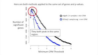
StatQuest Stats are going crazy. StatQuest Stats are going bonkers, baby. StatQuest Hello, and welcome to StatQuest. StatQuest is brought to you by the friendly folks in the genetics department at the University of North Carolina at Chapel Hill. Today, we're doing part two of our in-depth analysis of how edgeR and DESeq2 work. Specifically, we're going to talk about filtering out genes with low read counts, aka independent filtering, aka mitigating the multiple testing problem. Every time we do a statistical test, there's a chance that the conclusion is wrong. Psst. If this is news to you, check out the StatQuest on P values. In a nutshell, when we say P values less than 0.05 are significant, then we are also saying 5% of the time we will report a false positive. This isn't a big deal when we test one or two genes for differential expression because 5% of two tests is small, and it is unlikely we report a false positive. However, it's a big deal when we check every gene in the genome, about 20,000, to see which are misregulated in cancer cells. 5% of 20,000 equals 1,000 false positives. The good news is that FDR and the Benjamini-Hochberg method compensate for this problem. Psst. If this is news to you, check out the StatQuest on FDR. But there's another problem. To see what it is, let's look at an example. Let's imagine we have two separate distributions. On the Y axis, we have the probability of measuring different weights, and on the X axis, we have different weights in grams. The red curve represents the weights of mouse strain X. The blue curve represents the weights of mouse strain Y. If we weighed one strain X mouse, there's a high probability that the value will be near the middle of the red distribution. Likewise, if we weighed two more strain X mice, it is likely that those values will also be near the middle. Similarly, if we weighed three strain Y mice, there's a good chance those values will be near the middle of the blue distribution. A T test on these weights would result in a P value less than 0.05, and we would correctly conclude that the measurements came from different distributions. However, every now and then, we'll get overlapping values. In this case, the P value will be large. This is a false negative. Now, get a computer to take 1,000 samples from these distributions and do 1,000 T tests. Here's a histogram of the 1,000 P values that I got when I tried this at home. The T tests compared samples from two different, but overlapping, distributions. On the far left side of the histogram, we see 949 true positives, P values that are less than 0.05. However, we also predicted that sometimes the values would overlap, and we get P values larger than 0.05. This happened 51 times. So far, every single test we've done was supposed to result in a true positive and a P value less than 0.05. This is because every single test used samples from two different distributions. Let's make it more realistic by adding tests where there is no difference. We'll start with the 1,000 P values we already calculated using different distributions. Then we'll add 1,000 additional P values from samples taken from the same distribution. These P values should be greater than 0.05. But every now and then, say 5% of the time, we'll get something like this where the values are separated from each other and the P value will be less than 0.05. Now we have a histogram of 2,000 P values. 1,000 P values from the first bunch of tests where we had two separate distributions and 1,000 P values from the second set of tests where we took all the data from the same distribution. The 993 P values less than 0.05 are now a combination of 949 true positives from the first set of P values and 44 false positives from the second set of P values. Since only 4% of the P values less than 0.05 are false positives, we don't need to use FDR. But this is only because we made up the data. If it were real, we wouldn't know the percentage, so we'd use FDR. So let's use FDR and see what happens. After adjusting the P values for multiple testing, 846 FDR adjusted P values remained less than 0.05. 827 of the true positives survived. That's 89% of the original 949. And also 19 of the false positives survived. 2% of the 846 with FDR P values less than 0.05. Now, let's make it a little bit more like RNA-Seq and increase the number of P values to 6,000. We have the thousand P values from our first bunch of tests where we took the samples from different distributions. And we'll add to that 5,000 additional P values where the samples came from the same distribution. These additional 5,000 tests should give large P values most of the time. Here's a histogram of those 6,000 P values. There are now 1,215 P values less than 0.05. As before, 949 P values are true positives. But now, 266 are false positives. 22% of the P values less than 0.05 are false positives. That means it's time for FDR. After adjusting for multiple testing, only 256 FDR adjusted P values remained less than 0.05. 250 of the true positives survived. That's only 26% of the original 949. Six of the false positives survived. That's 2% of the 256 with FDR values less than 0.05. FDR is doing a great job limiting the number of false positives in the significant results, but it's not awesome at keeping the true positives. Now, let's increase the total number of P values to 11,000. 1,000 of those P values will be from the original tests, which were taken from two separate distributions, and 10,000 of those P values will be taken from the same distribution. And here's a histogram of those 11,000 P values. There are now 1,430 P values less than 0.05. As before, 949 P values are true positives, but now 481, or 34%, are false positives. After adjusting for multiple testing, only 56 FDR-adjusted P values remained less than 0.05. 54 of the true positives survived, only 6% of the original 949. Two of the false positives survived, 4% of the 56 with FDR values less than 0.05. Each time we increase the number of bogus tests, we reduce the number of true positive P values less than 0.05 that survived the FDR adjustment. Here's a graph of the data that we just generated. The green line represents true positives that passed FDR less than 0.05, and the orange line represents false positives that passed FDR less than 0.05. This graph shows that even though FDR can control the percentage of false positives that we report, regardless of the number of tests, it is in our interest to filter out bogus tests. It also suggests that there is room to improve the Benjamini-Hochberg method. So, get to it. We need something better. Both edgeR and DESeq2 have methods to filter bogus tests. The general idea is that genes with super low read counts are not informative. Thus, they can be removed from the data set. In other words, even if those genes are biologically interesting, it's hard to get accurate read counts if there are only one or two transcripts in one sample type and three or four in the other sample type. Before doing anything, edgeR recommends removing all genes except those with more than one CPM in two or more samples. CPM stands for counts per million. It compensates for differences in read depth between libraries. Let's quickly see how to calculate CPM. Here, we have a data set from a kidney. This data set has just over 5 million total reads. Here's the formula for calculating CPM. You take the reads for gene X in sample Y, and you divide that by the total reads in sample Y divided by 1 million. In this case, we plug in the total number of reads for our kidney sample into the bottom part of the equation. This gives us 5.32 in the denominator. Now, we put each gene's read counts into the numerator. Starting with the first gene, we put 65 in the numerator. This gives us a CPM value of 12.3 for the first gene. Now we plug in five for the second gene. And this gives us 0.9 CPM for gene number two. The reason why we scale the total read counts by 1 million is to keep the denominator from being too large. Otherwise, the resulting CPM values would be these tiny tiny tiny numbers with tons of decimal places and that's no fun to look at. Now that we have CPM values for all genes and all samples, let's remove all genes except those with more than one CPM in two or more samples. We'll start by examining gene one. Since it has two samples with more than one CPM in them, we'll keep gene one. Now let's look at gene number two. Again, since two samples have more than one CPM in them, we'll keep gene number two. Now let's look at gene number three. Since only one sample has more than one CPM, we'll filter this gene out even though that one sample has a lot of reads mapping to it. Now let's look at gene number four. Since the two samples with reads mapping to them have less than one CPM in them, we'll filter this one out. Now let's look at gene number five. This gene has reads in all four samples, but none are greater than one CPM, so we'll filter it out. Looking at gene six, this gene has greater than one CPM in two samples, so we'll keep it even though those two samples are from different tissue types. edgeR's method is simple, but you should be aware of how sequencing depth can influence it. For example, if you have 5 million reads mapping to a sample, the CPM scaling factor is 5 million divided by 1 million, which equals 5. If you have five reads mapping to a gene, it will have 5 / 5 = 1 CPM. If you have 80 million reads, then the scaling factor is 80. In this case, 1 CPM equals 80 reads. This might be too high. On the other hand, sometimes you need a larger CPM cutoff. For example, if you have 50,000 reads mapping to a sample, which isn't horrible for some single-cell RNA sequencing experiments, the CPM scaling factor is 0.05. If you have one read mapping to a gene, it will turn into 1 / 0.05 = 20 CPM. Even if this gene is transcribed at a biologically relevant level, and you only got one read because of the low overall counts, it is still in a very noisy range. Since CPM can change from data set to data set, how can we determine what a good cutoff is? Go with our gut? Look at real data? Let's look at real data. We're scientists, after all. To do that, I got a data set from a co-worker that has an average of 22 million reads per sample, four wild-type samples and four knockout samples. I then ran edgeR on it without filtering a single gene. This generated raw p-values. Lastly, I filtered out genes using different CPM cutoffs and then adjusted the P values. Here's what the data look like. On the Y axis, we have the number of genes with FDR less than 0.05. And on the X axis, we have the minimum CPM threshold. Zero means that there is no filtering at all. The recommended threshold is one. Because there are lots of reads, the suggested cutoff is too strict. It's actually worse than no filtering at all. Using a lower threshold identifies about 200 more significant genes. The moral of the story with edgeR is be careful. Try different CPM cutoffs after you've calculated the P values. Just so you know, I didn't come up with the idea to calculate P values before trying different cutoffs for the minimum CPM. That's how it's done in DESeq2. There are a few differences, though. So, let's talk about them. Difference number one. edgeR looks at individual samples and makes sure that at least two have more CPMs than the cutoff. edgeR looks at this gene and says, "Yep, those two samples are above the cutoff, so I'll keep the gene." In contrast, DESeq2 looks at the average normalized reads across all samples. DESeq2 looks at this gene and says, "Yep, the average of all four samples is above the cutoff, so I'll keep the gene." At this point, you're probably thinking, "Cool, I get DESeq2's approach. But what about genes with outlier measurements?" Liver 2 in this example might be an outlier measurement. This gene would not pass edgeR's criteria since only one sample has a large CPM. But what about DESeq2's? The average CPM for this gene is 5,000 / 4, which equals 1,250 CPM. This would probably pass the filter. That said, DESeq2 has an outlier detection method that we'll talk about in another StatQuest, but it only kicks in when there are more than two samples per category. Here are both methods applied to the same set of genes and P values. They both peak in the same region, and that's the most important thing. Both methods result in a similar cutoff. So now let's look at another difference. Another difference changes the X axis. DESeq2 plots the number of significant genes relative to quantiles instead of the minimum CPM cutoff. Zero on the X axis means that 0% of the genes are below the cutoff. 0.2 on the X axis means that 20% of the genes are below the cutoff. And 0.4 on the X axis means that 40% of the genes are below the cutoff. Quantiles are useful because, as we saw, CPMs depend on the sequencing depth, but quantiles are always quantiles no matter what. It doesn't matter if the library has 8 million or 80 million reads. 10% of the genes will always be less than the 0.1 quantile. But you don't have to choose. You can actually use both. Now let's talk about the third difference between edgeR and DESeq2. DESeq2 fits a curve to the points. This smooths out occasional bumps generated by random noise and makes the results more reliable. DESeq2 then locates the maximum location on the fitted curve. Lastly, the threshold is the maximum location on the curve minus the standard deviation between the fitted curve and the raw values. In other words, the first quantile that gets you within noise range of the peak becomes the CPM cutoff. If none of the raw values goes above the threshold, then no filtering is done. Okay. Now, we know how edgeR and DESeq2 filter genes. edgeR keeps genes that have more than the minimum CPM in two or more samples. DESeq2 keeps genes with the average CPM greater than the minimum CPM. It then plots the significant genes versus quantiles. It then fits a curve to those points, and the threshold is the maximum on that curve minus the noise. Now that you know, you can mix and match. Advice. If you use edgeR, figure out the CPM cutoff after you calculate the P values. It's easy to apply DESeq2's method to find the optimal CPM to edgeR's gene selection criteria. I've gone ahead and written template code and put it on my website, so check it out if you think you might want to do that. However, if you do, just make sure you cite both publications. If you use DESeq2, be careful of outliers when there are only two samples per category. Hooray! We've made it to the end of another exciting stat quest. Tune in for another exciting adventure in the land of statistics. Until then, quest on.