Dive into Deep Learning (Study Group): Convolutional Neural Networks | Session 6
Key Takeaways
This video introduces building blocks of Convolutional Neural Networks
Full Transcript
perfect i think we're good now i'm going to send it over to you okay very well [Music] okay awesome go ahead okay perfect so uh maybe a couple more minutes so two more minutes so briefly about myself um so i just put my linkedin and twitter if you want to connect feel free i'd be glad to connect uh briefly about me um i did my phd in engineering um i did um i i was doing i was doing machine learning but not the deep learning machine learning it just um just the traditional machine learning decision trees and all that building building healthcare healthcare applications after that i was faculty teaching engineering and then moved to industry works at different startups and all um if you are and and then right now and after working at different startups in computer vision and others nlp uh now i'm at nvidia as a deep learning instructor if you are on the path or this sounds uh something you know you're pursuing feel free to connect and um ask me anything okay um so uh maybe another minute or another minute or two for everyone to join in and then uh we'll start talking about cnns so again so um what will do the plan is we will do this today and uh next week so what happened is cnns they were proposing the 90s and then they kind of they fill out out of fashion because they weren't performing as well as other uh other machine learning algorithms in computer vision and then of course they came back after imagenet uh after imagenet uh 2012. so we'll be doing today we're going to be living in the 90s and uh and next uh but it's very but it's very important because there is pretty much the whole lecture is about well it's not a lecture so you said this it's a it's a study group right and i even have the i even have the book here uh open so if we need to to uh to reference to anything uh but what i was saying um yeah uh the convolution that that trick is that what we want to like mainly understand today so the goal by the end of this session we all wanna just okay when we see a cnn when we see a network like this we know we know all what's going on here if you already see it and you know uh you know for example you know this step here oh okay this is a convolution and this is a uh this is a kernel of size four and all that let me just just sit back and maybe you get to answer some of the questions on slack or uh but the goal eventually is you we are all comfortable building looking at this knowing what's happening between every layer so we're going to talk about different layers we want to understand what's happening between every layer because this is the base because everything that we'll do for example so we're going to see at the end of today we'll see like clinette which is the first which is the first proposed cnn back in the 90s but everything really builds up on that so if we really understand this one what comes next for example next week the next chapter i believe it's modern cnn so there is alex net and there is inception there i'm sure maybe maybe resnets uh and all those and really everything builds on on on on this everything actually built on the architectures before it but really everything builds on this so i think 607 so i think we can um go ahead and and start for for the questions i'm going to pause here and there and i'm so glad that elvis is also here so um you can probably post your questions on the chat maybe elvis can answer if he if elvis went out maybe during the pause want to just um ask me those i can answer those but we'll work it out okay um so yeah so starting um so next time um i'm gonna mention the different applications where cnns are used really the applications are are limitless you can think from self-driving to facial uh to facial emotional recognition to to work and with uh with maps to so many uh so many applications but if we were to summarize um maybe like the key ones like we usually we have these classifications and the common one is cash and dogs right uh and that's the the traditional the first one and then there is segmentation and you can see her segmentation is when we're going after sequential it's also based on so all these are based on cnns and then there are others okay okay and then there are others um like nerf style transfer and so forth and we'll dig more into more deaths when we talk about the different architectures okay cool so now um let's let's understand why why cnn why not so i i believe you've already talked about mlp so right now everyone is familiar with the musculated perceptron so why not just really process images which is a multi-layer perceptron right um so with that i'm going to ask you this question but before i had this slide which i already covered so and i wanted to present this slide at the beginning and now i'm probably we're going to look at it at the end but maybe now you look at it and say oh okay well i don't know what's going on exactly between here and here but um but to me being a good mate i have to make sure this by the end of this you you will certainly understand uh all the steps um here so i believe you already for example here we have the fully connected layers so i believe if we take the left side parts i believe here you're already fine but now today we're just adding cnn okay so we'll start with this question right why why not just use um multi-layer perceptrons with images and with that and uh with that um let's think of a scenario i think we have a one megapixel image and um so one one megapixel image and we have one hidden layer so if i had i was planning on using uh my notepad but i didn't want any glitches so i said i'll pass but if you do have a pen or something i think uh here and there i may say things and i think it's it's great if you have a pen next to you and you can like draw it down so for example here how about you draw uh one megapixel rgb image and then here one megapixel so it's a thousand by a thousand and rgb there's three channels so it's kind of like draw like a thousand by a thousand like three kind of like the cubes behind themselves so that and next to it here to the right you have a hidden layer and the hidden layer has a thousand units okay so if we're wondering what's the weight matrix if we use a fully connected layer again what's a fully connected layer meaning every node in those thousand is connected to all of the all of what all of the one thousand by one thousand times the three channels so thousand time thousand a million times three so three million per node so per node so that's like um right three uh three million three million times a thousand so that's like three billion so the weights metrics uh would have three billion parameters and we don't really want that we don't want that for many reasons we don't want that for example if you have all those if you have all those parameters first of all you need you need a huge data set right you need a huge data set to even train because the number of parameters is so big um second you need so much compute if you have all those parameters um uh you're most likely to overfit as well anyway so so this is the key so this is we're trying to kind of minimize all those never the 3 billion if we use the convolution it's going to be a lot less and now and now we'll see how is it going to be a lot less so that's the key so the key that we want to use high resolution images even more than this more than this uh one megapixel image and and this is just one image so now imagine if you have a data set that you have many many many images that so um so there's gonna be a lot more okay so so so that's why we use this convolution so let's understand what is this convolution and with that so i'm trying to follow the formats of the book there are different ways how anybody would like present this the cnns but since this is a study group about this book and i personally like the book for many reasons one of the main reasons is the book is actually updated all the time and not a lot of books are like that so that's that that's i think great about the book um so yeah so the format here and although that that you see is from the book um so that way you can even ask specific questions about uh paragraphs and maybe you have any um any any questions on i made sure i read the chapter so um uh so so what is the intuition okay so now we know the limitation the constraints are fully connected layer uh what is the intuition behind cnns and we'll get we'll get to the convolution in a second and the book they give this worries waldo example game and then they talk about translation in variance and locality and so here if we take this picture and we say where is waldo okay i was pointing with the monster as well though but if you look at it if you look at it uh okay wonder is here but really but really waldo the what what translation invariance is waldo doesn't really change if he's here or really here or at some other point and that's what translation invariance is so meaning that our network should really act or handle waldo the same in a way if no matter where he is in the image so that's pretty much the example that they give and locality we don't need for example these people here on the boat they don't they don't really provide much information for us to to to know much about waldo so what that means is we just need the pixels around waldo so maybe we just need a few pixels here and those can tell us and then like we can slide and those would tell us oh okay is this this password is dispatch world is this spanish no and that's locality and so these are the intuitions um behind cnn okay so let's let's uh delve more into them i was not planning on presenting math at the beginning of the lecture because i know that that may throw some of you off but but there is no really no reason to be thrown off on this one so this is again the equations that were shared in the book but um but yeah let's let's uh let's let's go through it so here now okay i said an mlp recap because you've already covered mlp so consider an mlp with a 2d image x so x is index k and l and there is a hidden representation uh age that's also it's in 2d again now if you have a pen and paper it would be really great uh to maybe draw some and by the way i may be going slow maybe there are some of you that are already very familiar with this but i i'm taking no assumptions maybe some of you are just getting through this so so if you already know all this you know just just bear with us it's gonna get more advanced uh as we go um so we have we have x so we're going to draw x it has indices k l and then also our h is in 2d so we're going to draw here on the right our h as in 2d and the indices for h are i n i n j so now what is the weight metrics between these two using mlp again mlp it's a fully connected layer mean in every a feature in our hidden representation is connected to all the input features okay and this is exactly why we have this weight symmetric metrics labeled by all these four indices i j and k l okay and it should be it should be good if you can actually draw the lines between them and actually um maybe next time i can just uh try it out on the notepad and and then share that with you if you guys all got it that's fine so um yeah so that that's pretty much it and so this is the mlp so this is something that you've already seen so nothing new here uh this is just a bias that we add and then here um if we say if we re-index this is just uh re-indexing we're gonna say k is i plus i plus uh i plus a and l is j plus b so we just replace that and same thing here here with it because we just replace that here because this is just a weight matrix we can just simply change it with another matrix and this is what we did here and here we said that this new matrix v is just same as this one so this is this is the one this is the one um yeah uh this is uh this is the one this is the one that that we had so i think this is clear if you have any questions about this uh please let me know i i'd be glad to represent this one okay so here based on multiplayer perceptron we have our input we have the met with the weight matrix and this is our hitter representation um we add some bias here okay uh next so now we're gonna talk about those two intuitions so how how are we gonna use those intuitions to really from this equation we're gonna derive now the new equation after convolution okay so now we're gonna go from a multi-layer perceptron something that we already know so here i believe we are all familiar with this one and now we're just going to add these two intuitions on top of this one so what was the first one the first one was translation in variance uh what's translation invariance again we said waldo doesn't really matter if he's here or here or anywhere right so so a shift in waldo a shift in our input should simply lead to a shift on the header representation okay what does that really mean that means that our weight matrix should not depend on i and j of the hidden representation okay and i'll just pause there so so now if going back to if you draw those two next to each other uh inj in the representation uh our weight matrix should not depend on the location of of of aldo so um so with this one here we can really just take off this inj from here and then with that we're just gonna be left with a and b okay and um and you know what i'm gonna open the chat and in the chat if you feel like hey um maybe maybe explain that's more please um okay okay cool awesome okay so this is what translation invariance is okay so uh now and this is very important why this is very important because here now if you already drew this you had all the nodes on the header representation connected to all to all of to all of the um to all of uh the input uh the the input features but now we're not gonna have that anymore uh we're actually gonna just have them linked to to only specific patches let's just say patches okay um maybe i can draw this the next time okay so so far we're here and um so these two so the the which metrics and this one did not depend on on i and j okay so now this is our new in our new equation and this is really what convolution is so this whole operation here this whole operation here is convolution and we're going to see more in detail what's his convolution and and again the book says that this is actually cross-correlation and not convolution which is exactly uh true and we will compare between what is the difference between convolution and cross-correlation and um okay uh i'm not going to look at the chart so maybe not to be too destructive uh okay are you referring to the output of the layer that we pass on to the next layer um why does v have a four indices uh okay so so we have four indices going back because from this one okay v i have four indices because we're really all that we did uh we really replaced this one this matrix here with just a different metric so here there is not much nothing changed and if you and if we uh because it's a multi-layer perceptron we have we have four indices um it doesn't depend on inj so with this we can just take off inj um i'm going to keep going and then in a bit i'm going to pause and take all the questions okay so now we have this um okay cool uh locality so what's locality locality again we said that this the waldo here does not depend on on what's happening here far away so we can only really look at the pixels really close to to his face to us all so what really represents aldo and that's exactly what this one uh what locality is and then we add this delta which we can think of as a threshold that we say you know what we're just going to look at between only here and here and we're only going to look at which cooling in here and here and so forth so anything outside so pretty much going back to the metrics anything outside uh of these pixels it's going to be zero okay um so we kept everything same so this is the equation that we got from the last the previous slide nothing added except now we're actually making our a within uh threshold and that threshold is what we call our kernel and i'm gonna and it's no worries if you are lost at any point uh i i i will go back and i will even draw that so it's fine if if it's fine if all this few equations didn't uh we can go through the book and i will revisit them again it's no worries but but this is the key here okay so i'm just explaining what translation invariance and locality are okay um okay so so so with that what is this cross-correlation which is also called convolution and this is and this is the part that that everyone okay so now maybe if you're lost okay now i hope you're not but now this is this is what cross correlation is so you have this kernel and this kernel comes from this threshold that we that this is the this is how we're relating the equations with this kernel so uh all that we do is we multiply and sum and so for example here so say this is we have this kernel this is again this is our input you can think of it as an image okay so it's like a 2d uh it's a 2d tensor you've been dealing now with tensors already so this is like a 2d sensor or a matrix we over lay this one here it's like we multiply and then we sum them up so if we uh and this is here you can see zero times zero one times one two times three three times four right if we add them up we're gonna get 19. okay now what we do we slide exactly as you see here we slide that to window to the right and then we get the 25 so so now if we slide it to the right we're just gonna get that kernel times what now times one two and four and five and then we'll get 25 and then after that one here it's good it goes down here uh so if you just want to code that it's like one for loop that's going uh over the columns and another for loop that goes down uh the rows okay that's pretty much what cross-correlation is and this is really what convolution is okay so a convolutional layer so now that's what cross-correlation a convolutional layer is simply is simply the cross correlation plus the bias so we do our cross correlation we get that that's the what we just seen on the previous slide and then when we add the bias to it that gives us the output and this is what we call a convolutional layer okay and uh instead of the when i wanna i'm gonna try this uh this way now uh to kind of even instead of trying to code later i'm gonna just try the code now like throughout how we go and then um okay so let's jump jump to the code okay so so okay so uh we we get this all of us so well all that we did we just multiplied and we got that okay cool so how the book um did that let's go and see um okay or uh what i can do [Music] we can actually have them so we can actually have them next to each other so that way we can um okay so this is where we talk so okay so let's implement this one uh let's let's implement this one so cross correlation okay i guess we'll go back to the cross correlation so cross correlation again uh is just two for loops right one going through the columns and then the other one going through zeros and that's exactly what uh what the code here is doing so to compute the cross correlation let me maybe uh zoom in there so to compute the cross correlation we have our kernel so this is what we could so this is the kernel again from the threshold we get this kernel we have this kernel that has a shape height and width and then we have our output outputs uh something here that i didn't mention what's the size what's the shape of our output it's the input minus the kernel size plus one okay input for example let's say for example here what's our input uh it's three three by three right so the height and h would be three and n w would be three minus again here they're the same the the the height and the width so two two so three minus two plus 1 that would give us 2 2 okay okay and uh so we specify the size of our y here and pretty much we just uh [Music] we just here we just multiply them we just multiply them and and then we just sum them okay and then this this same exact example the zero one two three four five here we can just uh do it as a as a 2d tensor here so we have just a 2d sensor and uh we do cross correlation with this kernel here same one and um and and we get the same results okay so i think that that's that's that's clear um okay so for the convolutional layer okay are you are you sharing two screens or are because we can only see one screen but it's very very small oh oh i'm shooting two screen oh okay the slides but we're not able to see anything else but it's very very small um how about now yeah now we're able to see yeah oh okay okay thank you for that yeah and you know elvis even even for the questions if if if anybody um if somebody says i'm very very lost then please please interrupt me and tell me if it's you know like i don't want to keep going and you know so um we want to make sure that yes we keep going but we want to like to take the questions as well anyways okay so thanks for that so all i was saying is i had these two pulled up next to each other now i believe you can see both screens and um i was just talking about uh what we just did here or what we just did um here how like okay we're computing the cross correlation and then we have our kernel shape the height and then we declare our y the shape of y is just that and this is exactly what we see here here the x shape minus h plus one okay and then a for loop going through the columns and a four loop going through the rows and then here we just multiply we just multiply and then sum and then that gives us our y okay and then this is the same exact example that the book presented here that we have here they just do it here and then you can see that the result is the same okay so we'll run that and okay so that was cross correlation so uh for the convolutional layer is just the same we all what do we say it's just same with but we just add the bias to it and that's all that we do here so we define this function which is pretty much just our cross correlation plus and our bias these two parameters here the words and bias and again all this is this is from the book and let's do the example of the book of the edges detection i have another another example that i like that i will present in a few slides but let's do the example of the book here uh they initialize uh they initialize this tensor with all ones so there are all ones and then they go and between two and six they put zeros okay and then they say and then now we have this kernel what's the size of this kernel it's uh one by two so what's this kernel uh so here we can think of one as being white and zero as being black what we're trying to do we're trying to detect the edges uh so crying all that we're trying to do is where where does this really change so what we're trying to do this kernel is trying to detect our vertical edges is there a vertical is there a vertical uh edge here between here and here no no no color change so now there's nothing oh yes there is a color change okay so we are we're expecting there to detect something is there color changing here no and so forth okay and so if we now apply the same cross correlation between this k and that that's exactly what we get we get the one here meaning that there was there was a edge detection between one and zero meaning going from white to black and then when we get the negative one here that means we detected uh change and edge direction from black to white okay um so that's all what that is and then i think they they say a question uh in the book i believe they say if you do the transpose and then uh can this detect horizontal and then um can this detect horizontal uh horizontal uh edges and this one would not detect horizontal adjusting for another text horizontal edges we want to why not change the kernel to be to really be just that okay okay okay so uh with that okay so with that talking about now so the key the key here are all about deep learning what we try to do we try to learn the waste matrix that's always you we visited the back propagation and all that it's all about finding those weights so and this is what they present here is okay now say that we have an input and then say that we have an output y um how do we go about finding the kernel okay and then here we already know the kernel size okay so we already know kernel is one by two how do we go find about finding the weights of the kernel um and this is where the back propagation comes right so and and that's what we have here so we have this 10 iterations that we're going to go over and then we do the convolution the 2d convolution of x that gives us our prediction y hat uh again this function that's just uh counts to d we get this prediction and then this is our loss right this is just the squared error between the prediction and the actual output and then here we zero the gradients before we do the back propagation and then we just update the weights and then we just it's right through that 10 times that's all that we're doing here and then by the end of this this should really have the weight of our kernel okay um let me zoom out let's see up there okay the error uh shape is invalid for uh oh okay uh let's see okay this should be fine okay so yeah so and then this is uh what we got uh 0.98 and negative one which is very similar to that kernel that we actually that we actually had at the beginning so so just straight forward so i believe since you've already maybe went through the first chapter so nothing nothing here um so very similar to the multi-layer perceptron how you would find those weights okay uh actually i think this is a good part a good point to make a pause and then i'll take uh questions now um actually the next the next point here okay so now i'm gonna just go to this window only so let me i'm gonna go now to my presentation slides okay um let me just go there so so yeah so yeah this is a good point to i'm gonna pause and take any questions and then keep going okay so um i'll see i'm looking at the chat right now say okay so um okay so there's a question here yes about the weight matrix so the question is if the weight matrix is directly replaced with the kernel in the convolution layer uh is the weight metrics so okay so so that's a good question so so usually for example when we start training like if you remember with the weight mattresses we always start with like random random weights right and then over time over time we update those weights so which is very similar to the kernel so eventually um yes you have the size of your kernel wherever that is three by three five by five and all that you're working on is you're actually updating oh well um uh uh so so you have you have uh the kernel so so yeah so uh that's what you're learning so so you're learning the the kernel the the kernel uh weights the the weights metrics um so um okay um yeah so um i hope i didn't confuse you there but yeah what i said what i said uh so yes so you already know you already know your kernel and then with the back propagation you just try to find what's what is the different every kernel you can think of that it's extraction a specific feature for example and then we'll see later we'll talk about channels but that's how you can think of it um okay uh what what are some other questions elvis cool that's a good explanation and i think someone mentioned it in the chat as well so i think that's pretty consistent okay um another question here so the question is by doing the convolution um aren't we reducing the size of the image yes exactly that's a very good point and that's why we have padding and exactly and we'll get to that that's a very good point and that's uh we'll get to that yes uh and also a question i think maybe later on you can answer but if you have a great time maybe so the initialization is the same as in a normal neural network like javier initialization so we will talk so uh so right now let's not worry about the the initialization uh right now you can for example if you used uh whatever initialization you used right now it's fine so if you use xavier for example or it's it's fine so for example at the end when we when we'll get to the learnet we will see for example which initialization will do and uh so for now it's fine just because you have a random insulin initialization right now okay one more one more question i think this is a good question um is there there there is i don't know if it's a question of the comment but i think the question is is there a way to define a criminal size just using the input data just using uh okay so so so with that so with that there are like good practices uh standards let's say so for example there are very common kernel sizes already so for example you'd find people uh usually using like a three by three a very common one or a five by five or even a seven by seven so these are the most the the common ones but getting a kernel size from the data um no i mean uh again again this is and uh this is this is a good point so here's the thing i'm sure you guys have talked about hyper parameters and parameters what's the difference between hyper parameters and parameters so the hyper parameters are things hyperparametered are things that we set right so you can think of your question that you asked me uh what's the size of my kernels what's the size of my kernel it's a hyperparameter so it is up to you and then anything that's up to you people have experimented with it what's the best one i'm one of when and same thing with that anything that comes to your mind as a learner as a hyper parameter from the learning rate to a kernel size to anything so and best practices five by five three by three seven by seven and it will even talk about why odd why not not even uh elvis any other any other uh question i think we're good now okay okay yeah yeah of course okay awesome so uh what's the difference between cross correlation and convolution uh they are pretty much the same uh just the kernel is flipped in convolution and this is what we see here so a b negative a and negative b and then here when i when we say the kernel is flipped it is flipped horizontally and it's also flipped vertically that's all the difference and then uh so if the kernel is symmetric the results will be identical and then here i have an example so for example and i took these screenshots um i think from a scanned book or something that i saw but they make the point so say you have this is your input and this is your kernel okay um and you see how here like there's w so think of some you will find it's being called kernel filter these are the two common ones and we'll see even later what's really even the difference between a filter and a kernel um but anyway so we have this and this is if we do our cross correlation this is what we get and i'm going to pause here by now by now you should be able to get this of course by yourself and then if we do a full convolution we're not gonna get this we get this okay that should make sense and you can just if you just get how you made the nine here you got it right because like you start here or this so this is a three by three so you start here three by three and then you slide you know uh you slide one stride or button to the right and then one to the bottom and then so and then so here you'll get all zeros and then you slide and so forth and then once you get here what's the first one that you get is when all the three here and three here so what the what the wood so i'm talking about i'm talking about this so which one will touch that to one first it's gonna be the nine and that's where the nine is here and so forth if you actually flip what we said convolution is just the kernel flipped horizontally and vertically so if we flip it actually one two three will be flipped it's gonna be three two one and also uh and also um vertically so it will actually end up something like that okay so it so this is actually what's going to be your kernel and if you do it and this is what you will get this is the result for conclusion okay um that's all so they're the same many so actually i took this from i took this from from this book that i have uh and i was reading it and this is fun but uh so i took it from this book if you know i don't see myself but i took it from this book and he says that um that's many libraries many machine learning libraries they implement cross-correlation but they call its convolution but but does it really matter it doesn't really matter why because what we're trying to learn we're trying to learn the kernel right the kernel that's what we're uh uh and and that's what we're focused on so it doesn't really matter but and and go and do some research you'll find some you know here and there but just uh but just know that the core of it is cross correlation okay there is this cool uh if you are um if if you've watched success ai and all by the way i was actually um i would do a shout out to all the fest ai fellows because um because i because when i first moved to san francisco actually uh the first thing that i joined was here uh at usf germany and and all these ai fellows were here so so anyways my point is he likes to show this one and i also really like it because it makes a point of edge detection but just like what we saw but even more so what we'll hear what we have so we have an image so we have an image and then you have the pixels of the image here okay so and then you have this is the kernel that we see so far we've been just looking at this two by two right so so far we've been looking at this really two by two here the the only difference is it's a three by three kernel okay and then although we do is we multiply this kernel with with you see this red things and then what we get as the result we get edge detection and that's all what's going on and so this is how hd section for example happens in images so we just related what we just seen on these numbers now to actually find an application back in the day uh edge protection was not done this way actually in a day education was done uh differently um but yeah so here you can uh and i've shared that you can come here and and play with it so what what we're here if you notice when we change this it just changes our uh kernel and by the change of our kernel then our multiplication with this image is just going to give us different things so we see for example how this left so sobel or sobel so here there isn't much difference between the the colors right uh so the reason there isn't but for example when you go close to the eyes with that you know we we find there is the edge detection and where is that coming from that's that's really just coming from the kernel okay um and you can see that this is kind of like a symmetric kernel this is kind of how it's really this one an edge detection kernel because it's kind of like one two one negative one negative two negative uh one okay uh so this is really cool so just go and play around with it and um also there is a second uh example here for it uh where you can actually play around with uh with changing even the values of your kernel you can give it any kind of value okay cool so um i think this because uh it's also it's always good to relate to we learned the theory to application so i think this is good so moving forward um okay um i'm gonna do another pause i'm gonna do another pause after four questions after after few slides so so far we've been talking only about a single input channel but in reality we we asked that question at the beginning rgb so rgb it's not a single channel it's so for example when we're talking about grayscale it's one one single channel but rgb is three channels right so we want to be able to deal with multiple input channels as well as multiple output charts okay and this is what we have here but really one with the cross correlation that we understood really that's the core of it so nothing changes so here okay we added the channel here a point that uh to make and i noticed here the kernel must have the same number of channels as the input okay so the channels in the kernel and why so that way we can perform we can do our cross correlation so this first uh channel of the kernel is going to go with our first channel here and then the second channel of the kernel is going to go with the second channel of the of our input we do our multiplication and then we just sum the whole thing and that gives us here a single output channel a single output channel okay so really nothing changed here uh you you can look at this one you can say oh okay i can multiply this and i sum them and i will get a 2 by 2 and then here i will get 2 by 2 and then i can sum them that's fine or if you sum them it's just just same really okay um okay so there was a single output channel how about multiple output channels and this is so now for example here we have this colored image so it's a it's uh it's an rgb image so we can think of it as a as a three channel image and we went from this uh we did convolutions and for forgets about all forgets about all this let's just focus on just this one here and and this here so we have this input with multiple channels with three channels and then here we have multiple output channels okay the only difference between what we've seen here and then what we see here on this one this is the difference if we take this one and we say let's add another kernel we're going to add another uh another kernel which we can now call a filter okay so we can still have we can say we can still say we have one kernel but this one kernel have two filters okay so with this one and maybe same as this one but maybe just different values here and that's going to give us what that's going to give us this one and it's going to give us another channel and if we have maybe three filters maybe if we have four filters for example so here we have four so we definitely had a kernel with four filters the four because we have four filters in our kernel here we're gonna get four output channels and that's all that's all that there is so now perfect now we understand this now when we look at we see this we know oh okay we just used four okay there are four uh these we call them feature maps oh there are four feature maps meaning we used four filters our kernel had four filters and i'll pause there and you see how we said feature map you see a feature map and the feature map really corresponds to like so this is one feature map you can think of it we can think as here we have four feature maps meaning what meaning every feature map is corresponding to a filter okay good meaning what meaning that filter is maybe detecting something so maybe one filter will detect the edges the horizontal edges maybe another filter will detect the vertical edges maybe and and and and so forth and this is in the lower levels and you can think the more the more deeper you get then that's how for example let's say a face is detected because there were filters that maybe they were detecting something specific maybe the eyes eventually on a much higher level a level and so forth okay um so now uh so now okay we are at least fine we have this input and then when we look at this okay we just say okay we know how we got here we had like three channels inputs here but now here we actually have four output channels how did we get four output channels oh because our kernel had four filters oh okay that's fine and and but but then if i ask you okay the kernel had four filters but how many channels did every filter have oh you'll say well that will depend on how many channels were on my input oh your input was an rgb image it's three channels okay so every filter had three channels okay so we had four filters and every filter had three channels within it okay cool you say for example here because here we only have two channels okay i believe that should be clear the last point here to make this is just like a special case of this multiple output channel this is just a one by one convolutional layer and you may even say when would this really be used but it is used and there is a very popular architecture called inception which i believe it should be uh i didn't fully uh go through the modern convolution but it should be i'm expecting achieving on that chapter and one component of it uh uses the one by one convolution and so when when do we really use this so okay so for example here i'm gonna step back just based on what we learned what do we have here oh okay we have an input that has three channels so our kernel must have three channels okay perfect but how many filters do we have we have two filters okay we have two filters mean and what meaning we're gonna get two channels out and that's what we have here we get two channels out what's and then we do the cross correlation between the kernel and what between our kernel and then we slide it here we just slide one by because there is just one so we're just gonna get the same size so and this is how this one by one is used so we actually the the input size does not change but what's really changed is the number of channels oh how does that change based on how many filters we have on our kernel okay so if you uh so and this is how i also noted here so when do we use this one by one convolutional layer is to adjust the number of channels between the network layers and to control the the model complexity okay uh so you can think of it now again as we said this whole filter maybe is detecting something this is detecting something and then you got this maybe now you want you can go from here now and then you can go to maybe a single output channel and so forth okay but i i i believe so far so clear um we're going to go through the code and after the the code we'll we'll take questions okay um let's let's do the the double screen like earlier um okay let's see one second uh elvis well i'm doing this please ask me if if there is anything any questions i just listen okay so far so good okay thanks okay let's uh have now uh these two next to each other and then we'll run the code okay so uh we're gonna run here we're gonna run the multiple input channels we're gonna run the multiple output channels and the one by one okay so let's go back to that multiple one okay um okay so we've already done the cross correlation so that's good so here what we have okay we define this there is nothing here that changed this is our this is our uh cross correlation and then here we just use this zip which just uh zips our input with our kernel um you know if if you're if you're not familiar with this one you can just uh you can just do it by itself and then and and then and then see for example and then see what you get so for example um i'll have to do it if i want to do it i'll do it after i'll do it after this one so if we zip that you can see that it took so for example here it took the first one the first tensor it's it uh zips it with this one and then it will take the the second tensor here and it will just zip it with this one okay and then it's pretty much just performs the cross correlation on them just as before before we only saw a single example right a single one now it's just both and it just adds them so it just sums everything so there is really nothing here new uh it just now sums everything together and that's how we got here our 56 72 104 and 121 um okay uh okay so for the multiple output channels uh yeah what we do is we just stack them stack the results together so here the multiple article channels so what we're going to do is we're going to use this example that we have here we're going to use this same one here what did we say now if we want to have multiple output channels we just want to have more filters right so we're just going to have we still want to have like a 2d uh two channels in but more okay and this is what we do here so for example here we take our kernel and then we add plus one to it and then we add plus two to it actually so this one i um there is something called broadcasting you probably seen this seen it uh already so all that it does it's broadcast this plus one it adds that to the whole um to the whole kernel so actually for example so here what we will do is actually yeah we can actually um we can um and you know you can just so this is our first one zero one two three one two three four and then it just adds one so it just adds one now we have this is our second filter and this is our third filter and then we just and then we just um do our regular uh cross correlation okay and then we get three output channels one two and three so now this is the multiple output channels and then the last one this one the convolutional layer was just a special case of of a multiple output uh output uh multiple uh output layer and here what they're doing pretty much with the book they said they uh they related this to really using a fully connected layer which is which is the same so and this is how they so if you so you see like this is a new function that's pretty much that it just uses the matrix multiplication the dot products pretty much and then they show how doing it this way is just the same as you see this is the new function that they did and they should do within it this one this way is the same as if we do it our other way you see how here like for example when you subtract them from each other the results would be smaller than this that's true um and if you would like to think how is that here what they did is they reshaped them so you can you can think of this okay so maybe this is like uh a homework or not a homework just just a practice kind of thing so how about uh if you have any doubts here what i would personally suggest how about you draw this draw this and see how they actually they will shape this into for example if you look at here it's going to be and what happens here okay so what kind of matrix multiplication is here for example for this example it's going to be here 2 by 3 k is going to be now 2 here you see if we reshape it is going to be 2 by 3 which is just these two and then our x is going to be when we reshape it it's going to be three by nine okay now we can actually do matrix multiplication two by three times uh three by nine and that's going to give us two which is two for the output channels and nine and then we're gonna have to reshape exactly and that's what what they do here the reset and nine again so it's actually um so it's actually the height and width to the entry okay uh so they'll do it for now um and moving on moving on we're just gonna do some more recap or we're gonna go even more practical now so i'll pause here and we'll take any questions or yeah if not we'll keep going okay cool so now now uh you should be seeing uh okay yes now you should only be seeing this one okay so so far so good right so okay so now let's put everything together what we've learned so far um okay okay so so we have the fully connected layer for example here if we have our input as one by the three we have our weight matrix and then we get a number from the dot if we just do the dot product we're gonna get 10 outputs here right okay uh this is just using the fully connected layer so nothing new here now let's just take this and do it now in 3d right for example okay so now we want just from this one so this is something that you probably implemented on the last chapters now we're going to go into 3d so now for example we have a 32x32 image and then we have three because it's a color and that's why red green blue so it's an rgb and i have to actually to give credit for where i got this slide from so i got them from justin i believe his name justin johnson he um he was the one he was one of the tas who taught the stanford convolution uh but i will actually post a link here but uh that's where i got this i really like the visualizations here because they make the point so we talked about the filters right so now we have this filter that is this is a single filter that it's it has a size five by five by three okay y d3 because it has to match the input channels okay and now when we convolve it it's just kind of like overlay it and then we just slide it slide it all over okay and then you can then you can do the math and then know what's the output so what's so if you remember actually from that equation that we saw what's that so what's the output that we're expecting if you remember if we have an input image and then we have a kernel size we can predict we can say we can say that's the output so the output we say it's the input minus the kernel plus one so for example here it will be 32 minus five plus one right so it will be 28. so the output here that we're expecting is 28 by 28 and that's what we get here at 28.28 yes this is what we call an activation map if we call it an activation map uh if we have an activation function added to it okay so so this is or we can just call it a feature map okay okay perfect so that's what we know what we have how about now if we have a second filter we've seen that already now we're just gonna have another feature map here and then we have and and so forth and if we have many features filters for example here if we have six filters we're just gonna do the same you see uh we're just gonna do six first and you see how like the annotation in here six filters three we can call this like cn channels in so six filters three channels five by five and then we get six output channels 28 by 28. okay cool okay so we've seen all that of course we add bias to it every filter would have its own bias so we add the bias to with every filter we had a bias okay um now we can have more batches so here we're talking about a single image we can have many images right and so forth and so the conclusion here if when i like give so we had n number of batches uh for example a batch would have five images so our end would have would be five if it is an rgb it will be three the height and width of that okay and then what's the our uh c out c out will be just the number of filters that we have and then the c n here is from our input and then the width and the height of the kernel and uh so now we actually now we can say just how before we said oh okay well this is what we're expecting 28 km from 32 minus uh 32 minus five plus one then we can make a generalization of this and we'll make that generalization of this now and even when we'll add padding and straws and also and all that there is an equation for that okay so now if we stack convolutional layers perfect so now i will ask a question so if we stack so okay so now we have that right uh this is something so now when we look at this we should all be familiar with oh okay we have this input this is a 32 by 32 with three channels okay it's an rgb and when we look at this we know what's going on here three filters three three channels five by five we're expecting this answer or so forth we can apply it and this is what a cnn is but the question now i would say is can this this is something all nerd so i'm going to step back and say all neural networks they actually aim to do one thing they aim for one thing there is a theorem a very popular it's called the universal approximation theorem and this is and this is what deep learning this is what neural networks is all about what is this universal approximation theorem it pretty much says that any function can be approximated with enough data and enough inputs let's say okay so enough inputs with enough inputs we can approximate any function okay that's that's the goal that's all our goal with all these architectures even with the high non-dimensionality and all that the goal is we're just trying to approximate functions to either classify different objects or to the regression or anything but most of what we're working with is non-linear right most of the functions if one of the really you know linear would just take you so much so here i would ask you the question if we just do this is this can can really this mimic a non-linear function meaning what meaning for us to actually to have to to to have some mapping non-linear meaning like we gotta have some non-linearity inside and really on convolutional here so far we're just multiplying and adding there is no nonlinearity there and this is where this is this is why i wear my shirt this is where really you comes okay so then that's really right real you you have this linearity that you really introduce after every output and that's uh and that's and that's how that's how we get a non-linear um a non-linear uh approximation that we're going for okay and i hope that is very clear and exactly and this is where the slide shows so we have the conc layer and we have our conv layer and then we add our activation function here which makes uh our output noun non-linear and this is exactly what we're looking for okay perfect so this is this is okay if we got so far here we are in very good shape now um this is now this is going to be like um very easy if i were to ask you this uh um if you have a 56 by 56 you can think of its image or whatever don't think of it as an image because you can say oh well how is that 64. well yes the rgb the inputs will be three image but sometimes when we are in the middle layers you can have something of like this size for example you can have something of um of uh here channels in 64. so this is cn channels in 64. so if we have our channels 64 and 56 156 and i say we're gonna do a one by one convolution with 32 filters so let's pause there a one by one convolution with 32 filters what's the x exit output size i'll ask you then every filter how many channels does it have for us to do the cross correlation every filter has to have 64 channels in it right okay so what's the expected size the expected size would just be 56 56 32 okay 32 because now the number of filters became our channels out okay so uh i'll pause here now we're going to talk about padding and stride and pulling these are just spatial dimensions you see like how earlier they said that there was a good question how like applying all the convolution definitely like shrinks the size and you know um so padding now comes and we're gonna talk about all that but i'll pause here and we can take any questions elvis if there is a question please no i didn't see any new questions so okay perfect i think we can move forward okay um so uh padding has tried and pulling uh exactly because the outputs get uh shrinks very fast for example especially if we use if we use uh kernels that are like for example here for example if we start by 32 by 32 and then we use a five by five kernel after just one okay we're gonna get uh 28 by 28 and after a few layers we even get four by four and uh because of this and because of this um we would like to introduce padding so padding is just pads zeros to the outside of our inputs okay and so for example if we have this three by three input here we pad it by zeros all around there and then we do our cross correlation and then instead of before if we did not have the padding what would be the expected output it would be just two by two but now we actually get a four by four okay so so um so straightforward there um so now again same way how we try to predict the output shape uh the output shape now we're just gonna add the padding the padding to the the height and the width uh that's gonna that's gonna be our output and the common choice i come a very common choice what's the pattern size it's the kernel minus one so for example if our kernel is three if our current e3 a typical choice would be three minus one would be two meaning we're gonna add one one to the right and the one to the left if for example if our kernel is five what we'll do here is five minus one it's four so we're gonna just add two to the left and two to the right okay uh this is a good point here to say this is why odd num when the kernel size is odd it works well because that way we can add even number of we can add even number of paddings to the right and to the left but if the kernel size is even when we do this and then we split by two one of the sides will actually have one more than that than the other okay and the stride uh stride is kind of like you can we can think of it as the the the other way around so you see how padding is actually so we keep that uh dimension uh not to reduce as fast actually strike sometimes maybe you want to reduce the dimension um the dimensions as fast and this is what for example here when we use stride and this is for example here but you can see it's pretty much we just skip couple couple uh slides here so for example here a stride of three for the height and the stride of two for the width so for example we will start here right so our kernel is overlaid here we do cross correlation here but instead of sliding it just one we're going to slide the two we're gonna slide the two for the weight so the next one actually will be here will there be another one no there will not be another one because if we slide another one yes we're gonna cover only one but we're not gonna cover the other one so for us we have to for for this one to be calculated we have the kernel has to cover everything and here's three for the height so we actually instead of actually going only down once we can actually go down three times okay and then and then you can imagine how like doing it this way it would really shrink our input size okay and this is how we really we can change the spatial dimension either like really growing them or really uh shrinking them um on on on a hard pace even because like even a kernel of just a kernel really shrinks them but strides does even more okay same way we tried to do uh to to say what's the output shape um this is what we had before and then what we just do we add now destroy to it and these are again these are taken from the book and we said that the typical choice would be just the kernel minus one and that's what we have here uh this is a typical choice right uh not not not always but this is a and then if we replace this one on on our equation we're just gonna get this one here and here if the height and width are divisible by stripes the output will just be the input over the stripe so for example if we have an input of eight by eight and then we say the stride is two our output will just be four by four and the lesson is pulling so pull in uh there are two types of coolant so pool and again when we talk about pool and point is uh and this is actually uh maybe even in interviews or what is pool and or pool is just down sampling in one word pulling is just down sampling um uh for example here there are two main types of pulling [Music] there is max pooling and there is average cooling and all that it does there is no there is no convolution here or anything but we have our window and then we just we just um we just take so this is our window for example two by two and then we just take the max from it okay that's our max coolant so for example here four and then we slide it and then what's the max here it's five and then so forth the average will just do the same but it's just gonna average them instead of taking the max uh and you can see how it says down sampling for example here it's scaled down from 224 by 224 to 112 and to 4812. okay um and then same thing here uh same thing here so this is an example of max cooling and this is this is an equivalent uh example of average spawning okay so what we'll do we'll go through the code and then if there are any questions after the code we'll we'll we'll we'll take those questions and the last thing that we'll cover will be the learner's architecture and we're certainly ready for it afterwards we have covered so far okay so let's now go back to the code and look at how padding and stride and cooling were implemented okay and i will share okay okay great so um tighten first so um so padding so i i hope everything now is everyone is following maybe accept those maybe uh even those uh initial equations those were fine but uh i think uh if you are lost at any point uh we'll have some time at the end that you can ask okay so um apply one pixel padding on all sides so this example of padding supplies one pixel heading on all sides so let's see here so we start with um okay we have a reshape here okay so we will reshape it because we want to add remember that batch and the number of channels okay and uh we do our cons here and then we reshape it here okay so we fully shape it uh if we're gonna just take out now uh the batch and uh the number of channels so for instance here we have our x is of size 8 by 8 and then when we apply this with okay so i did so this is lower scale so here this is so when we look at this here what are we what are we seeing we've seen that our kernel size is 3. meaning our uh height and width of the kernel is three by three and our padding here is one okay so meaning we padded our input by one to the right one to the left one above and one at one below so with that when we run this let's say if we do not have any padding let's say let's say if we do not have any padding what's the expected output here it would be like the eight minus three plus one so we're expecting six by six but because we have added one never expected now it's the same okay so really straightforward right but all these is very really important for for what we'll see next uh as we as we go and then so when a kernel has different height and width sitting different padding numbers for height and width can make outputs have dimensions same dimensions as input so here our current size the height is different than the width the height is five and the width of three and if we want to make the output the same as the the input then we can just add two and one so these the padding will also be different okay uh the stride uh we talked how destroyed we would just uh for example here two and again i'll pull up the destroyed here you can see how the stride would just uh uh with here so it's like it it skips right it's by how much do we slide our window and then here we have our padding to one and then our strike to two and then here we got four by four so um how did we even get this four by four you can do the math or you can what did we say here if it is divisible by the stride for example 8 by 8 yes it is divisible by 2 so or merit to the output shape will be just 4 by 4. okay and uh same thing here we have a kernel size that has a different shape and then here we can also pad with different numbers to the right and to the left and this is what we do here and even if our kernel is different we are able to get the same we are able to get a matching size on the height and the width because our paradigm is different uh lastly for pulling what did we say pool and there is max pool and average coolant and this is what the book here they show and pretty much you would just take the same thing it's going to be two for loops again these are just uh implementations of the book right um so this is not you know you usually you would just call this function right so so you'd have just uh affordable for your columns and for look for your rows and then you would just uh take the max over um this is how you would just slide your window and then you would just take the max if you're going for max pool and then you would just take the average or the mean if you're going for your average cooling and uh for example this one this example here the zero one two three four five this is exactly what they showed here and then when you have a window a pull in window of size two two right you just go and you get your uh max pool and this is what we get here four five seven and then if we do the average that's what we get okay so so right now uh so oh we covered all the main components of um of really of convolution and so forth here this slide here i'm gonna move now to this um to show in that only now we're ready actually to build our first architecture and the book they uh chose lynette um so so so this is just like a a summary of you remember how it talks about the different sizes um so this is just a generalization of everything so if we have our input the numbers of channels in the height and width the hyper parameters right and this is your common settings three by three uh kernel five by five kernel one by one kernel okay um the number of filters dictates the number of channels out we have padding we have stride um so this is our weight matrix which will be and and so so yes so so see how this weight matrix now is channels out channels in the kernel height and width so this is for this type of convolution and then maybe we'll get to talk later there are different types of convolution for example maybe one day you wanna you wanna start you wanna say you know what okay i'm gonna pause here and maybe just you know just step on the side and just say something maybe practical maybe you're gonna say you know it's okay now you got the convolution very well but but maybe you wanna maybe you wanna have a light you want to have a light model so what i mean is maybe you actually you're doing deep learning on edge devices if you're doing deep learning on edge devices the weight matrix matters a lot so so if you can really reduce this and still be able to to achieve the same performance that'd be great okay and there are other ways to do convolution that maybe we can see later or if you can look them up for example there is one called depth wise convolution and i'm sure because we have got so far until here if you just go through this by yourself you know exactly how depth wise convolution is doing and you can for example pick that and then you can work it out and then for example you can calculate the number of parameters because this is the number of parameters right and then the more parameters you have the more compute you need so you can actually maybe compare you can get the parameters from this one and maybe you can get the parameters using this same convolution but just it's slightly done differently you know steps and then wise and then you can compare the two so yeah so there are difference but again the core is the convolution and then here the output size we have the height and the width and this is the general form of our output shape of the height and width based on the initial the input height the kernel size the padding and the stride and this is all between currencies plus one okay so uh we got now to lynette and uh we're just going to talk about it and then we're going to see its implementation that the book presented on the fashion imminence um so here so here now you see maybe maybe maybe before maybe before our today's session maybe if you look at this you wouldn't know exactly what are all these numbers representing but i hope by now you look at them and you know exactly what's going on but there is a tricky kind of thing here that this i just took it from the from the book but there is something tricky for this with this uh this image but if you get it you know very well that so for example here we have a 28 by 28 image so if we apply so if i tell you you know what i'll tell you uh we applied a five by five kernel if i just tell you that we have a 28 by 28 image and we just apply the 5x5 kernel what's our output what are we expecting what's the size of our output it's not going to be 28 by 28 right so there has to be something that must have that we have done into this and this is so this is uh lynette so to answer that question he added he padded so he padded two uh to the right uh two to the left to the right and two all over and that's how for example so the input really is 32 by 32 and then the current the current here is five by five so now when you actually 32 and with the current of five by five 32 minus five plus one you get a 28 and then you have how did we get again this six channels out meaning our kernel simply had six filters um so by the way so lunata architecture proposed in uh by ian lacun i'm sure you all know him uh durian award of last year or the year before uh so the the one of the main the first successful applications because um but then and then why it died what kind of like the cnns they kind of like they weren't they didn't keep that momentum primarily because they needed a lot you see like how all this they needed a lot of data to train on and that's so a lot of data a lot of data and that's now where we have a lot of data and also a lot of gpu power and with all that we can actually you can even do more high resolution images we can even now you know how the the billion parameters that all the new models really have okay so now going and looking at this we say okay by the way so this is a single channel and we say okay we have a single channel but our output has many channels okay well that's probably because we use many filters here and then you know the size here and then here we apply coolant back then there wasn't uh max pulling was not proposed so it was just average pulling and then and then you do another count layer and then you do pull in and then here you just go from here to like a dense layer you just pretty much flatten this into a test layer and so forth and then here you have three fully connected layers okay so um so this is again uh how uh how the book details it and this is exactly what the architecture is so we start with the image exactly how we said we have a conf layer of uh 5.5 size the heat added two with six filters and then we do average pulling the pool side the window size two by two the stride and usually this is a good point here to mention that usually usually the stride would be the same size as the pool window so exactly here pulled by two usually uh and then here there is no padding you see how here we padded here there is um can you see you can see my my screen right i just want to make sure yes okay and so forth and so so right now i feel we're all and again to make this of course to make all this to make to make all this the the non-linear rights because we're trying so we we have to add the sigmoid so for example now we're talking about real you back then there was just uh the sig mode was was the activation function and this and this is a and this is how we go about it okay so now let's go to the last part and just go over the code for this one and um so for this one um okay so we're running this on collab and um okay so i believe you can see my collab window now and um i'll zoom in okay so we already so i believe you're already it's just uh sequential so we're just putting layers sequentially um a convolutional layer then we applied our silver we apply our sigmoid then we apply an average pooling then a convolution the sigmoid and so forth and then here we specify the the kernel size the stride and so forth and lastly here after we flatten that we just have to be fully connected uh layers okay uh that's so here with the book they say they just wanted to try this out with just a random a random input that's 28 by 28 and this is they just show they just print out the the different um the the structure they just put out the network here and this is exactly what we went through through uh on the slide okay so now to apply this on the fashion mnist we specify a batch size a large batch size here 256. um again batch sizes they're usually power of twos so you can 64 256 and so forth um okay so once we load that i believe you already maybe have done if you have done this for ml for ml performance layer perceptrons this will be just the same so the this is for our test so this is eval is for our uh test and then we'll have our training and training will be down and then here we're making sure we're making sure that we're using our gpu um okay this is this is a d2l so this is a function in there that that's probably just adding an accumulator there and then here we're just so we're copying the data here to the gpu and then we're just calculating the accuracy so when are we going to call this so we're going to call this function when we're going to evaluate the accuracy of our test set okay so um for training we initialize our weight i think somebody asked a question earlier of for instance here we're initializing our weights using sevier and um we specify that we're using our gpu and then the optimizer is sgd the loss is cross entropy we have an animator to show our results here at the bottom that's where the animator we start we have a timer and then now we go and iterate through our number of our epochs which we which we will specify later um we tell the model we're gonna train we zero out our gradients we copy the data to the gpu we predict our y hat we calculate the loss and then we back propagate and then we update the step and then we get we keep track of our training accuracy here and then we keep track um we keep track of our training accuracy there and if that this is for the animator when are we going to plot that pretty much and then here the test accuracy we go back and we use the evaluate accuracy gpu function that we declared up top and these are just some printouts to print out and then we just specify here the learning rate uh and the number of epochs and then we retrain and then it just trains and pretty much now we have trained our model that it's prediction with an accuracy of 80 percent say on our first cnn network and um and i will pause here and we'll take questions and any discussions anything specifically on the chapter that i may have skipped maybe feel free to ask me and any anything i know i'll share okay just waiting for questions if anyone has sometimes it takes a little while for people to answer a question but there was one question here um i think it was about the number of input filters okay no that's not the part so they're talking about something about sizing i say i understand how stride padding affect the size of the output but i'm not clear on how the filters change the output channels okay okay so so um okay so he's saying that um he is clear on how the stride changes the output right but not quite on how that is affecting how the filters change the output channels yes okay so so the filters so for example we can go to any to any to any of these so the filters the number of filters is the number of our channel outputs and okay so um to even explain that more for example here we have two filters so we get two output channels okay i mean it's like it's like we take one filter it's like think of it as like uh this one here where for example this one here we only have one filter a filter that has two channels so we only got one now when we add another filter we'll get another output channel and then we can think that that's why a channel right a channel is related to a filter that's why sometimes you can even relate channels to the features they're extracting that's why we can really relate the feature wherever the eyes on the high level or maybe the edge detection on the lower level to we can relate them to the filters but actually we can relate them to even the channels so maybe the channel space actually next time there is something that i may have skipped here which is a receptive field and um and that can maybe help visualize this excellent i think that was pretty clear um so another question could you discuss additional applications of cnns in addition to the visual space so so yeah um you know so so cnn is like for example uh they can even be used as a 1d so cnns can be used even for text if you would like and so that's like 1d and instead of just rgb they can even be used with more than even three dimensions so they're like they're still visual but it's visual but there are more dimension than just rgb uh for example um for example the geospatial maps and all those so those they have like an extra dimension uh so that's for besides visual um also also also here's another way how you can so here's please guys here's another way how uh i would like you to also think of cnns so think of cnns not only only for computer vision but think of them also as feature extractors meaning what meaning you see like how we have this okay we may extract something from whatever input we have for example that question that somebody just asked something else than visual whatever you have here for example you may have you may apply cnn and then once you get here to the end maybe your output is not necessarily computer vision for example you can feed this so you can think of this as a feature map that you can feed it to other networks you can maybe feed this into lstms for example you can feed this into uh the different things so so yes they are used for computer vision but they're also you can think of them as feature extractors and then you may want to use those features on other things okay and all those are very good questions yeah they're very good everyone is so curious about the cnns there's another one i think another question here say it says stride pulling kernel always reduce size and padding always increases size but filters can either increase or decrease depending on our choice is that the right assumption so so that's another that's another good point so you see so so here is um you see the deeper the deeper we go what here what do you notice the deeper you go you notice that the dimensions really the the size gets smaller but the filter the channels which are the filters the channels out gets larger and this is just this is what had this is just kind of like best practice what has been found to work best we're like kind of like sacrificing that spatial dimension right because we're making smaller but we're actually getting more features from it and you can think of now those channels out so for example here so for example let's say for example here we have four right we're looking at this one here we have four so you can think now maybe all this more like for example here maybe we have eight or sixteen each one of them maybe is getting like so maybe one of this one here is kind of like representing the i this is intuitively because really they're not independent like that they're all in a way related to each other but we can think of them like that so we are sacrificing we are making them smaller but for us to make them smaller we're actually we have to also uh keep some of that uh some of that feature information and that's how we do by increasing the the filters which is that the channel the channels out there yeah okay cool um i don't see any other so yes there's some other comments there but no questions anyone else has any questions to ask i think you you finished with your presentation right salim yes yes uh this is yes uh this is it and and again so actually this is now the basics and then and now that we all can look at this one and then we all got it uh i believe now we've just taken this now to our next level and to from alex ned to the to the latest ones um we're all going to be very comfortable with this all that i would say is these equations if you have i'm gonna i'm gonna check the slack uh the dyer the our slack channel if you have any still any doubts about this uh please let me know i will share maybe like a diagram or something of of here how like we went how we had like here four indices and the four indices were really it doesn't really this translation invariant so it's not these are very these are intuitions behind cnns this is how we went from all that multi the number of a huge weight metrics to a much much smaller now weight matrix which which we call the kernel yeah everyone is so happy about the presentations they really love that apparently well i'm i'm sure then now it's going to be even more fun right because now that we understand all this now uh you can go and well what i would what i would suggest i know for example i went very fast through this so what i would suggest go back through this at least maybe now start changing maybe small things okay we said this is sigmoid okay now we know that really you works better than sigmoid right start changing things like that uh okay here they used average pooling okay do max pooling and and and and just and and and now you have enough now you have enough to start building things and then it and i believe the the the even more passion would come when you actually build something and you can and you can share it with friends and others and so for example for that section i'm going to wrap up with this so what i would wrap up is my experience with deep learning with machine learning and after and then you know i'm i'm no expert we're always to learn and learn all the time but you get to realize that um you could realize that yes deeply machinery is important but if it doesn't make it to production if others don't use your application you know that's so what i would say but it doesn't have to be complex it can be just something like this and there are tools for example i really like this tool called streamlit which you can just easily build an app for it a web app or something so just use like just tools like this where you can just build something and you can just post it and and things like that and and yeah so that's that's what i would say cool thanks alimon that's a great suggestion again towards the end someone actually asked in our previous session um whether you know if anyone was interested in doing a presentation on using streamlit to do a very basic demo or something like that i think that'll be great and if somebody really you know like you said you are encouraging people to try it i think that's a good challenge and if someone gets to do it i think that would be a great presentation i think as a project that would be awesome um we are going to have a project towards the end of the the whole program so i think that would be a great time to to think about it and to start to do some investigation there so thanks for that suggestion yeah and this is like even uh personally with like colleagues and and all that even like i don't know if anybody is looking for jobs or not but when you are looking for jobs and you go and you even say that hey okay i built this even if it's not too complex but you know i built a streamlit app for it or just whatever app like for example back we used to use flask but now i i feel like streaming is even more friendlier and all that uh you can just use that and that's perfect you may even pull it up on your phone be like hey here it is and once you have even your streamlets on the app you can you can even put it on a darker image and then you can start playing so i i think so this is this is kind of like you know um so yes uh deep learning and machine learning and all well yeah but you share share with friends share with others yeah okay thank you thank you very much yeah see you guys next week thank you bye you
Original Description
Deep Learning Study Group - Session #6 - Convolutional Neural Networks
In this session, we introduce the building blocks to convolutional neural networks.
Entire playlist: https://www.youtube.com/playlist?list=PLGSHbNsNO4ViFXawDmx-kEz7zGziOpNSb
You can find more information about the deep learning study program and upcoming sessions here: https://github.com/dair-ai/d2l-study-group
Watch on YouTube ↗
(saves to browser)
Sign in to unlock AI tutor explanation · ⚡30
Playlist
Uploads from Elvis Saravia · Elvis Saravia · 19 of 60
1
 2
2
 3
3
 4
4
 5
5
 6
6
 7
7
 8
8
 9
9
 10
10
 11
11
 12
12
 13
13
 14
14
 15
15
 16
16
 17
17
 18
18
 ▶
▶
 20
20
 21
21
 22
22
 23
23
 24
24
 25
25
 26
26
 27
27
 28
28
 29
29
 30
30
 31
31
 32
32
 33
33
 34
34
 35
35
 36
36
 37
37
 38
38
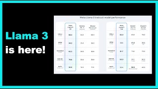 39
39
 40
40
 41
41
 42
42
 43
43
 44
44
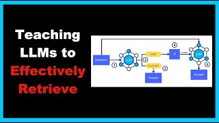 45
45
 46
46
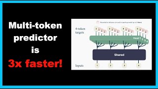 47
47
 48
48
 49
49
![[LLM NEWS] AlphaFold 3, xLSTM, OpenAI's Model Spec, DeepSeek-V2, OpenDevin CodeAct 1.0](https://i.ytimg.com/vi/fzg84wDevkQ/mqdefault.jpg) 50
50
 51
51
 52
52
![[LLM NEWS] KANs, Gemma 10M Context, OpenAI Updates?, Automatic Prompt Engineering, Tokenizer Arena](https://i.ytimg.com/vi/ehLVG1gcmqE/mqdefault.jpg) 53
53
![[LLM News] GPT4-o, Project Astra, Veo, Copilot+ PCs, Gemini 1.5 Flash, Chameleon](https://i.ytimg.com/vi/p7xQRIHWG_M/mqdefault.jpg) 54
54
 55
55
 56
56
 57
57
![[LLM News] xAI Series B, Codestral, LLM Guide, AutoGen Course, Symbolic Chain-of-Thought](https://i.ytimg.com/vi/BBhLELGj77k/mqdefault.jpg) 58
58
 59
59
 60
60

101 ways to solve search (by Pratik Bhavsar)
Elvis Saravia
TLDR Generation of Scientific Documents | ML Interview #1 with Isabel Cachola
Elvis Saravia
Sentiment Analysis: Key Milestones, Challenges and New Directions
Elvis Saravia
Discriminative Adversarial Search for Abstractive Summarization (by Thomas Scialom)
Elvis Saravia
Question Understanding: COVID-Q: 1,600+ Questions about COVID-19
Elvis Saravia
Getting Started with NLP
Elvis Saravia
Building tools and frameworks for large-scale social media mining (by Dr. Juan M. Banda)
Elvis Saravia
TextAttack: A Framework for Data Augmentation and Adversarial Training in NLP
Elvis Saravia
Dive into Deep Learning (Study Group): Introduction to Deep Learning | Session 1
Elvis Saravia
Dive into Deep Learning (Study Group): Multilayer Perceptrons | Session 4
Elvis Saravia
How I read and annotate ML papers
Elvis Saravia
Keep Learning ML (Session 1) | DSV, CompLex, Modern tools for emotions
Elvis Saravia
Dive into Deep Learning (Study Group): Preliminaries | Session 2
Elvis Saravia
Keep Learning ML #2 | Language-conditioned policy learning, Effective ML Testing, EagerPy
Elvis Saravia
Dive into Deep Learning (Study Group): Linear Neural Networks | Session 3
Elvis Saravia
Dive into Deep Learning (Study Group): Multilayer Perceptrons | Session 4
Elvis Saravia
Keep Learning ML #3 | Contrastively Trained Structured World Models
Elvis Saravia
Dive into Deep Learning (Study Group): Deep Learning Computation with PyTorch | Session 5
Elvis Saravia
Dive into Deep Learning (Study Group): Convolutional Neural Networks | Session 6
Elvis Saravia
Dive into Deep Learning (Study Group): Modern CNNs | Session 7
Elvis Saravia
101 ways to solve neural search with Jina
Elvis Saravia
(Hopefully-Reusable) Life Lessons for PhD Students in NLP
Elvis Saravia
How to save the world and forward your career in 5 easy steps | Women in NLP Talks
Elvis Saravia
Prompt Engineering Overview
Elvis Saravia
Getting Started with the OpenAI Playground
Elvis Saravia
LM-Guided Chain of Thought
Elvis Saravia
Elements of a Prompt
Elvis Saravia
Reasoning with Intermediate Revision and Search with LLMs #chatgpt #ai #llms #science #programming
Elvis Saravia
General Tips for Designing Prompts
Elvis Saravia
Efficient Infinite Context Transformers #ai #machinelearning #research #llms #science
Elvis Saravia
Best Practices and Lessons Learned on Synthetic Data for Language Models #ai #machinelearning #genai
Elvis Saravia
Reducing Hallucinations in Structured Outputs via RAG #chatgpt #ai #llms #programming
Elvis Saravia
Basic Prompt Examples for LLMs
Elvis Saravia
LLM In Context Recall is Prompt Dependent #llms #ai #chatgpt #machinelearning
Elvis Saravia
Zero-shot Prompting Explained
Elvis Saravia
RAG Faithfulness #llms #ai #gpt4
Elvis Saravia
Understanding LLM Settings
Elvis Saravia
Llama 3 is here! | First impressions and thoughts
Elvis Saravia
Llama 3 is Here! #ai #llms #llama3
Elvis Saravia
Microsoft introduces Phi-3 | The most capable small language model?
Elvis Saravia
Microsoft introduces Phi-3! #ai #llms #microsoft
Elvis Saravia
Make Your LLM Fully Utilize the Context #ai #llms #machinelearning
Elvis Saravia
When to Retrieve? #ai #llms #machinelearning
Elvis Saravia
Training an LLM to effectively use information retrieval
Elvis Saravia
State-of-the-art open-source LLM judges #ai #machinelearning #gpt4
Elvis Saravia
Better and Faster LLMs via Multi-token Prediction
Elvis Saravia
AlphaMath Almost Zero #ai #science #machinelearning
Elvis Saravia
SWE-Agent | An LLM-based Software Engineering Agent
Elvis Saravia
[LLM NEWS] AlphaFold 3, xLSTM, OpenAI's Model Spec, DeepSeek-V2, OpenDevin CodeAct 1.0
Elvis Saravia
LLM-powered tool for web scraping #ai #chatgpt #engineering
Elvis Saravia
Learn about LLMs in this NEW course #ai #chatgpt #engineering
Elvis Saravia
[LLM NEWS] KANs, Gemma 10M Context, OpenAI Updates?, Automatic Prompt Engineering, Tokenizer Arena
Elvis Saravia
[LLM News] GPT4-o, Project Astra, Veo, Copilot+ PCs, Gemini 1.5 Flash, Chameleon
Elvis Saravia
Enhancing Answer Selection in LLMs #ai #machinelearning #engineering
Elvis Saravia
On exploring LLMs #ai #promptengineering #chatgpt
Elvis Saravia
Transformers Can Do Arithmetic with the Right Embeddings #ai #machinelearning #engineering
Elvis Saravia
[LLM News] xAI Series B, Codestral, LLM Guide, AutoGen Course, Symbolic Chain-of-Thought
Elvis Saravia
PR-Agent #ai #gpt4 #software
Elvis Saravia
Extracting features from Claude 3 Sonnet
Elvis Saravia
Has prompt engineering been solved?
Elvis Saravia
Related Reads
📰
📰
📰
📰
How to Choose the Best Deep Learning Model for Medical Imaging
Medium · Deep Learning
Another Way to Read Neural Geometry
Medium · Data Science
Another Way to Read Neural Geometry
Medium · Deep Learning
Building My First Neural Network From Scratch with PyTorch: A Journey on the Dry Bean Dataset
Medium · Deep Learning
🎓
Tutor Explanation
 DeepCamp AI