TensorFlow 2.0 Complete Course - Python Neural Networks for Beginners Tutorial
Skills:
Neural Network Basics90%
Key Takeaways
Covers the fundamentals of TensorFlow 2.0 and Python neural networks for beginners
Full Transcript
hello everybody and welcome to an absolutely massive tensorflow slach learningartificial intelligence course now please stick with me for this short introduction as I am going to give you a lot of important information regarding the course content the resources for the course and what you can expect after going through this now first I will tell you who this course is aimed for so this course is aimed for people that are beginners in machine learning and artificial intelligence or maybe have a little bit of understanding but are trying to get better but do have a basic fundamental knowledge of programming and python so this is not a course you're going to take if you haven't done any programming before or if you don't know any python syntax in general it's going to be highly advised that you understand the basic syntax behind python as I'm not going to be explaining that throughout this course now in terms of your instructor for this course that is going to be me my name is Tim some of you may know me as Tech with Tim from my YouTube channel where I teach all kinds of different programming topics and I've actually been working with free code camp and posted some of my series on their Channel as well now let's get into the course breakdown and talk about exactly what you're going to learn and what you can expect from this course so as this course is geared towards beginners and people just getting started in the machine learning and AI World we're going to start by breaking down exactly what machine learning and artificial intelligence is so talking about what the differences are between them the different types of machine learning um reinforcement learning for example versus neural networks versus simple uh machine learning we're going to go through all those different differences and then we're going to get into a General introduction of tensorflow now for those of you that don't know tensorflow is a module developed and maintained by Google which can be used within python to do a ton of different scientific Computing machine learning and artificial intelligence applications we're going to be working with that through the entire tutorial series and after we do that General introduction to tensorflow we're going to get into our core learning algorithms now these are the learning algorithms that you need to know before we can get further into machine learning they build a really strong Foundation they're pretty easy to understand and implement they're extremely powerful after we do that we're going to get into neural networks discuss all the different things that go into how neural networks work how we can use them and then do a bunch of different examples and then we're going to get into some more complex aspects of machine learning and artificial intelligence and get to convolutional neural networks which can do things like image recognition and detection and then we're going to get into recurrent neural networks which are going to do things like natural language processing chatbots text processing all those different kinds of things and finally ended off with reinforcement learning now in terms of resources for this course there are a ton and what we're going to be doing to make this really easy for you and for me is doing everything through Google collaboratory Now if you haven't heard of Google collaboratory essentially it's a collaborative coding environment that runs an IPython notebook in the cloud on a Google machine where you can do all of your machine learning for free so you don't need to install any packages you don't need to use pip you don't need to get your environment set up all you need to do is open a new Google collaboratory window and you can start writing code and that's what we're going to be doing in this series if you look in the description right now you will see links to all of the notebooks that I use throughout this guide so if there's anything that you want to be cleared up if you want the code for yourself if you want just text based descriptions of the things that I'm saying you can click those links and gain access to them so with that being said I'm very excited to get started I hope you guys are as well and let's go ahead and get into the content so in this first section I'm going to spend a few minutes discussing the difference between artificial intelligence neural networks and machine learning now the reason we need to go into this is because we're going to be covering all of these topics throughout this course so it's vital that you guys understand what these actually mean and you can kind of differentiate between them so that's what we're going to focus on now now quick disclaimer here just so everyone's aware I'm using something called Windows Inc this just default comes with Windows I have a drawing tablet down here and this is what I'm going to be using for some of the explanatory Parts where there's no real coding um just to kind of illustrate some Concepts and topics you now I have very horrible handwriting I'm not artistic whatsoever programming is definitely more of my thing than uh you know drawing and doing diagrams and stuff but I'm going to try my best and this is just the way that I find I can convey information the best to you guys so anyways let's get started and discuss the first topic here which is artificial intelligence now artificial intelligence is a huge hype nowadays and it's funny because a lot of people actually don't know what this means or they try to tell people that what they've created is not artificial intelligence when when in reality it actually is now the kind of formal definition of AI and I'm just going to read it off of my slide here to make sure that I'm not messing this up is the effort to automate intellectual tasks normally performed by humans now that's a fairly vague definition right what is considered an intellectual task and you know really that doesn't help us too much so what I'm going to do is bring us back to when AI was create first created to kind of explain to you how AI has evolved and what it really started out being so back in 19 50 there was kind of the question being asked by scientists and researchers can computers think can we get them to figure things out can we get away from just hardcoding and you know having like can we get a computer to think can it do its own thing so that was kind of the question that was asked and that's when the term artificial intelligence was kind of coined and created now back then AI was simply a predefined set of rules so if you're thinking about an AI for maybe like Tic taac toe or an AI for chess all they would have had back then is predefined rules that humans had come up with and typed into the computer in code and the computer would simply execute those set of rules and follow those instructions so there was no deep learning machine learning crazy algorithms happening it was simply if you wanted the computer to do something you would have to tell it beforehand say you're in this position and this happens do this and that's what AI was and very good AI was simply just a very good set of rules or a ton of different rules that humans had implemented into some program you could have ai programs that are stretching you know half a million lines of code just with tons and tons and tons of different rules that have been created for that AI so just be aware that AI does not necessarily mean anything crazy complex or super complicated but essentially if you're trying to simulate some intellectual task like playing a game that a human would do with a computer that is considered AI so even a very basic artificial intelligence for a tic tac toe game where it plays against you that is still considered Ai and if we think of something like Pac-Man right where we have you know our little ghost and this will be my rough sketch of a ghost and we have our Pac-Man guy who will just be this well would we consider this ghost AI what it does is it attempts to find and kind of simulate how it would get to Pac-Man right and the way this works is just using a very basic pathf finding algorithm this is nothing to do with deep learning or machine learning or anything crazy but this is still considered artificial intelligence the computer is figuring out how it can kind of play and do something by following algorithm so we don't necessarily need to have anything crazy stupid complex to be considered AI it simply needs to just be simulating some intellectual human behavior that's kind of the definition of artificial intelligence now obviously today AI has evolved into a much more complex field where we now have machine learning and deep learning and all these other techniques which is what we're going to talk about now so what I want to start by doing is just drawing a circle here and I want to label this circle and say a I like that so this is going to define a AI because everything I'm about to put inside of here is considered artificial intelligence so now let's get into machine learning so what I'm going to do is draw another circle inside of here and we're going to label this circle ml for machine learning now notice I put this inside of the artificial intelligence Circle this is because machine learning is a part of artificial intelligence now what is machine learning well what we talked about previously was kind of the idea that AI used to just be a predefined set of rules rules right where what would happen is we would feed some data we would go through the rules by and then analyze the data with the rules and then we'd spit out some output which would be you know what we're going to do so in the classic example of Chess say we're in check well we pass that board information to the computer it looks at its sets of rules it determines we're in check and then it moves us somewhere else now what is machine learning in contrast to that well Machine learning is kind of the first field that actually figuring out the rules for us so rather than us hardcoding the rules into the computer what machine learning attempts to do is take the data and take what the output should be and figure out the rules for us so you'll often hear that you know machine learning requires a lot of data and you need ton of examples and you know um input data to really train a good model well the reason for that is because the way that machine Learning Works is it generates the rules for us we give it some input data we give it what the output data should be and then it looks at that information and figures out what rules can can we generate so that when we look at new data we can have the best possible output for that now that's also why a lot of the times machine learning models do not have 100% accuracy which means that they may not necessarily get the correct answer every single time and our goal when we create machine learning models is to raise our accuracy as high as possible which means it's going to make the fewest mistakes possible because just like a human you know our machine learning models which are trying to simulate you know human behavior can make mistakes so to sum that essentially machine learning the difference between that and kind of you know algorithms and basic artificial intelligence is the fact that rather get that rather than us the programmer giving it the rules it figures out the rules for us and we might not necessarily know explicitly what those rules are when we look at machine learning and create machine learning models but we know that we're giving some input data we're giving the expected output data and then it looks at all of that information does some algorithms which we'll talk about later on that and figures out the rules for us so that later when we give it some input data and we don't know the output data it can use those rules that it's figured out from our examples and all that training data that we gave it to generate some output okay so that's machine learning now we've covered Ai and machine learning and now it's time to cover neural networks or deep learning now this circle gets to go right inside of the machine learning right here I'm just going to label this one NN which stands for neural networks now neural networks get a big hype they're usually usually what the first you know when you get into machine learning you want to learn neural networks you're kind of like neural networks are cool they're capable of a lot but let's discuss what these really are so the easiest way to define a neural network is it is a form of machine learning that uses a layered representation of data now we're not going to really understand this completely right now but as we get further in that should start to make more sense as a definition but what I need to kind of illustrate to you is that in the previous example where we just talked about machine learning essentially what we had is we had some input bubbles which I'm going to Define as these we had some set of rules that is going to be in between here and then we had some output and what would happen is we feed this input to this set of rules something happens in here and then we get some output and then that is what you know our program does that's what we get from the model we pretty much just have two layers we have kind of the input layer the output layer and the rules are kind of just what connects those two layers together now in neural networks and what we call Deep learning we have more than two layers now I'm just trying to erase all this quickly so I can show you that so let's say and I'll draw this one another color because why not if we're talking about neural networks what we might have and this will vary and I'll talk about this in a second is the fact that we have an input layer which will be our first layer of data we could have some layers in between this layer that are all connected together and then we could have some output layer so essentially what happens is our data is going to be transformed through different layers and different things are going to happen there's going to be different connections between these layers and then eventually we will reach an output now it's very difficult to explain neural networks without going completely in depth so I'll cover a few more notes that I have here um essentially in neural networks we just have multiple layers that's kind of the way to think of them and as we see machine learning you guys should start to understand this more but just understand that we're dealing with multiple layers and a lot of people actually call this a multi-stage information EXP exraction process now I did not come up with that term I think that's from a book or something but essentially what ends up happening is we have our data at this first layer which is that input information which we're going to be passing to the model that we're going to do something with it then goes to another layer where it will be transformed it will change into something else using a predefined kind of set of rules and weights that we'll talk about later then it will pass through all of these different layers we different kind of features of the data which again we'll discuss in a second will be extracted will be figured out will be found until eventually we reach an output layer where we can kind of combine everything we've discovered about the data into some kind of output that's meaningful to our program so that's kind of the best that I can do to explain neural networks without going onto a deeper level I understand that a lot of you probably don't understand what they are right now and that's totally fine but just know that they are layered representation of data we have multiple layers of information whereas in standard machine learning we only have you know one one or two layers and in artificial intelligence in general we don't necessarily have to have like a predefined set of layers okay so that is pretty much it for neural networks there's one last thing I will say about them is that they're actually not modeled after the brain so a lot of people seem to think that neural networks are modeled after the brain and the fact that you have neurons firing in your brain and that can relate to neural networks now there is a biological inspiration for the name neural networks and the way that they work from you know human biology but it is not necessarily modeled about the way that our brain works and in fact we actually don't really know how a lot of the things in our brain operate and work so it would be impossible for us to say that neural networks are modeled after the brain because we actually don't know how information is kind of happens and occurs and transfers through our brain um or at least we don't know enough to be able to say this is exactly what it is a neural network so anyways that was kind of the last point there okay so now we need to talk about data now data is the most important part of machine learning and artificial intelligence neural networks as well and it's very important that we understand how important data is and what the different kind of parts of it are because they're going to be referenced a lot in any of the resources that we're using now what I want to do is just create an example here where I'm going to make a data set that is about students final grades in um like a school system so essentially we're going to make this a very easy example where all we're going to have for this data set is we're going to have information about students so we're going to have their midterm one grade their midterm 2 grade and then we're going to have their final grade so I'm just going to say midterm one and again excuse my handwriting here it's not the easiest thing to write with this drawing tablet and then I'll just do final so this is going to be our data set and we'll actually see some similar data sets to this as we go through and do some examples later on so for student one which we'll just put some students here we're going to have their midterm one grade maybe that's a 70 their midterm 2 grade maybe that was 80 and then let's say their final was um like their final term grade not just the mark on the final exam let's give them a 77 now for midterm 1 we can give someone a 60 maybe we give them a 90 and then we determine that the final grade on their exam was let's say an 804 and then we could do something with maybe a lower grade here so 40 50 and then maybe they got a 3 um 8 or something in the final grade now obviously um we could have some other information here that we're omitting maybe there was some exam some assignments whatever some other things they did that contributed to their grade but the problem that I want to consider here is the fact that given our midterm one grade and our midterm two grade and our final grade how can I use this information to predict any one of these three columns so if I were given a student's midterm one grade and I were given a student's final grade how could I predict their midterm two grade so this is where we're going to talk about features and labels now whatever information we have that is is the input information which is the information we will always have that we need to give to the model to get some output is what we call our features so in the example where we're trying to predict midterm 2 and let's just do this and uh highlight this in Red so we understand uh what we would have as our features our input information are going to be midterm one and final because this is the information we are going to use to predict something it is the input it is what we need to give the model and if we're training a model to look at midterm one and final grade whenever we want to make a new prediction we need to have that information to do so now what's highlighted in Red so this midterm 2 here is what we would call the label or the output now the label is simply what we are trying to look for or predict so when we talk about features versus labels features is our input information the information that we have that we need to use to make a prediction and our label is that output information that is just representing you know what we're looking for so when we feed our features to model it will give to us a label and that is kind of the point that we need to understand so that was the basic here um and now I'm just going to talk a little bit more about data because we will get into this more as we continue going and about the importance of it so the reason why data is so important is this is kind of the key thing that we use to create models so whenever we're doing Ai and machine learning we need data pretty much unless you're doing a very specific type of machine learning and artificial intelligence which we'll talk about later now for most of these models we need need tons of different data we need tons of different examples and that's because we know how machine learning works now which is essentially we're trying to come up with rules for a data set we have some input information we have some output information or some features and some labels we can give that to a model and tell it to start training and what it will do is come up with rules such that we can just give some features to the model in the future and then it should be able to give us a pretty good estimate of what the output should be so when we're training we have a set of training data and that is data where we have all of the features and all of the labels so we have all of this information then when we're going to test the model or use the model later on we would not have this midterm 2 information we wouldn't pass this to the model we would just pass our features which is midterm one and final and then we would get the output of midterm two so I hope that makes sense that just means data is extremely important if we're feeding um incorrect data or data that we shouldn't be using to the model that could definitely result in a lot of mistakes and if we have incorrect output information or incorrect input information that is going to cause a lot of mistakes as well because that is essentially what the model is using to learn and to kind of develop and figure out what it's going to do with new input information so anyways that is enough of data now let's talk about the different types of machine learning okay so now that we've discussed the difference between artificial intelligence machine learning and neural networks we have a kind of decent idea about what data is and the difference between features and labels it's time to talk about the different different types of machine learning specifically which are unsupervised learning supervised learning and reinforcement learning now these are just the different types of learning the different types of figuring things out now different kind of algorithms fit into these different categories from within artificial intelligence within machine learning and within neural networks so the first one we're going to talk about is supervised learning which is kind of what we've already discussed so I'll just write supervised up here again excuse the handwriting so supervised learning now what is this well supervised learning is kind of everything we've already learned which is we have some um features so we'll write our features like this right we have some features and those features correspond to some label or potentially labels sometimes we might predict more than one information so when we have this information we have the features and we have the labels what we do is we pass this information to some machine learning model it figures out the rules for us and then later on all we need is the features and it will give us some labels using those rules but essentially what supervised learning is is when we have both of this information the reason it's called supervised is because what ends up happening when we train our machine learning model is we pass the input information it makes some arbitrary prediction using the rules it already knows and then it Compares that prediction that it made to what the actual prediction is which is this label so we supervise the model and we say okay so you predicted that the color was red but really the color of whatever we passed in should have been blue so we need to tweak you just a little bit so that you get a little bit better and you move in the correct direction and that's kind of the way that this works for example say we're predicting you know student's final grade well if we predict that the final grade is 76 but the actual grade is 77 we were pretty close but we're not quite there so we supervise the model and we say hey we're going to tweak you just a little bit move you in the correct direction and hopefully we get you to 77 and that is kind of the way to explain this right you have the features you have the labels when you pass the features the model has some rules that it's already built it makes a prediction and then it Compares that prediction to the label and then retweets the model and continues doing this with thousands upon thousands upon thousands of pieces of data until eventually it gets so good that we can stop training it and that is what supervised learning is it's the most common type of learning it's definitely the most applicable in a lot of instances and most machine learning algorithms that are actually used use a form of supervised machine learning a lot of people seem to think that this is you know a less complicated less Advanced way of doing things that is definitely not true all of the different methods I'm going to tell you have different advantages and disadvantages and this has a massive Advantage when you have a ton of information and you have the output of that information as well but sometimes we don't have the luxury of doing that and that's where we talk about unsupervised learning so hopefully that made sense for supervised learning um tried my best to explain that and now let's go go into or sorry for supervised learning now let's go into unsupervised learning so if we know the definition of supervised learning we should hopefully be able to come up with the definition of unsupervised learning which is when we only have features so given a bunch of features like this and absolutely no labels no output for these features what we want to do is have the model come up with those labels for us now this is kind of weird you're kind of like wait how does that work why would we even want to do that well let's take this for an example we have some axis some axes of data okay and we have like a two-dimensional data point so I'm just going to call this let's say x and let's say y okay and I'm going to just put a bunch of dots on the screen that kind of represents like maybe a scatter plot of some of our different data and I'm just going to put some dots specifically closer um to other ones just so you guys kind of get the point of what we're trying to do here so let's do that okay so let's say I have this data set this here is what we're working with and we have these features the features in this instance are going to be X and Y right so X and Y are my features now we don't have any output specifically for these data points what we actually want to do is we want to create some kind of model that can cluster these data points which means figure out kind of you know unique groups of data and say okay so you're in group one you're in group two you're in group three and you're in group four we may not necessarily know how many groups we have although sometimes we do but what we want to do is just group them and kind of say okay we want to figure out which ones are similar and we want to combine those together so hopefully what we would do with an unsupervised machine learning model is pass all of these features and then have the model create kind of these groupings so like maybe this is a group maybe this is a group maybe this is a group if we were having four groupings and maybe if we had two groupings we might get groupings that look something like this right and then when we pass a new data point in that could we could figure out what group that was a part of by determining you know which one it is closer to now this is kind of a rough example it's hard to again explain all of these without going very in depth into the specific algorithms but unsupervised machine learning or just learning in general is when you don't have some output information you actually want the model to figure out the output for you and you don't really care how it gets there you just want it to get there and again a good example is clustering data points and we'll talk about some specific applications of when we might even want to use that later on just understand you have the features you don't have the labels and you get the unsupervised model to kind of figure it out for you okay so now our last type which is very different than the two types I just explained is called reinforcement learning now personally reinforcement learning and I don't even know if I want to spell this because I feel like I'm going to mess it up reinforcement learning is the coolest type of machine learning in my opinion and this is when you actually don't have any data you have what we call an agent an environment and a reward I'm going to explain this very briefly with a very very very simple example because it's hard to get too far so let's say we have a very basic game you know maybe we made this game ourselves and essentially the objective of the game is to get to the flag okay that's all it is we have some ground you can move left or right and we want to get to this flag well we want to train some artificial intelligence some machine learning model that can figure out how to do this so what we do is we call this our agent we call this entire thing so this whole thing here the environment so I guess I could write that here so environment think I spelled that correctly and then we have something called a reward and a reward is essentially what the agent gets when it does something correctly so let's say the agent takes one step over this way so let's say his a new position is here I just don't want to keep drawing him so I'm just going to use a DOT well he got closer to the flag so what I'm actually going to do is give him a plus two reward so let's say he moves again closer to the flag maybe I give him now plus one this time he got even closer and as he gets closer I give him more and more reward now what happens if he moves backwards so let's erase this and let's say that at some point in time rather than moving close to the FRA the flag he moves backwards well he might get a negative reward now essentially what the objective of this agent is to do is to maximize its reward so if you give it a negative reward for moving backwards it's going to remember that and it's going to say okay at this position here where I was standing when I moved backwards I got a negative reward so if I get to this position again I don't want to go backwards anymore I want to go forwards because that should give me a positive reward and the whole point of this is we have this agent that starts off with absolutely no idea no kind of you know knowledge of the environment and what it does is it starts exploring and it's a mixture of randomly exploring and exploring using kind of some of the things it's figured out so far to try to maximize its reward So eventually when the agent gets to the flag it will have the most the highest possible reward that it can have and then next time that we plug this agent into the environment it will know how to get to the flag immediately because it's kind of figured that out it's determined that in all of these different positions if I move here this is the best place to move so if I get in this position move there now this is again hard to explain without more detailed examples and going more mathematically and all of that but essentially just understand we have the agent which is kind of what the thing is that's moving around in our environment we have this environment which which is just what the agent can move around in and then we have a reward and the reward is what we need to figure out as the programmer a way to reward the agent correctly ly so that it gets to the objective in the best possible way but the agent simply maximizes that reward so it just figures out where I need to go to maximize that reward it starts at the beginning kind of randomly exploring the environment because it doesn't know any of the rewards it gets at any of the positions then as it explores some more different areas it kind of figures out the rules and the way that the environment works and then we determine how to reach the objective which is whatever it is that it is this is a very simple example you could train a reinforcement model to do this and you know like half a second right but there is way more advanced examples and there's been examples of reinforcement learning like of AI pretty much figuring out how to play games together how to it's it's actually pretty cool some of the stuff that reinforcement learning is doing and it's a really awesome kind of advancement in the field because it means we don't need all this data anymore we can just get this to kind of figure out how to do things for us and explore the environment and learn on its own now this can take a really long time this can take a very short amount of time really depends on the environment but a real applic of this is training AI to play games as you might be able to tell by kind of what I was explaining here and yeah so that is kind of the fundamental differences between supervised unsupervised and reinforcement learning we're going to cover all three of these topics throughout this course and it's really interesting to see some of the applications we can actually do with this so with that being said I'm going to kind of end what I'm going to call module one which is just a general overview of the different topics some definitions and getting a fundamental knowledge and in the next one what we're going to be talking about is what t Tor flow is we're going to get into coding a little bit and we're going to discuss um some different aspects of tensor flow and things we need to know to be able to move forward and do some more advanced things so now in module two of this course what we're going to be doing is getting a general introduction to tensorflow understanding what a tensor is understanding shapes and data representation and then how tensorflow actually works on a bit of a lower level this is very important because you can definitely go through and learn how to do machine Learning Without kind of gaining this information and knowledge but it makes it a lot more difficult to tweak your models and really understand what's going on if you don't you know have that fundamental lower level knowledge of how tensorflow actually works and operates so that's exactly what we're going to cover here now for those of you that don't know what tensorflow is essentially this is an open-source machine learning library it's one of the largest ones in the world it's one of the uh most well-known and it's maintained and supported by Google Now tensorflow essentially allows us to do um and create machine learning models and neural networks and all of that without having to have a very complex math background now as we get further in and we start discussing more in detail how neural networks work and machine learning algorithms actually function you'll realize there's a lot of math that goes into this now it starts off being very kind of fundamental like basic calculus and basic linear algebra and then it gets much more advanced into things like gradient descent and some more regression techniques and classification and essentially you know a lot of us don't know that and we don't really need to know that that so long as we have a basic understanding of it then we can use the tools that tensorflow provides for us to create models and that's exactly what tensorflow does now what I'm in right now is what I call Google collaboratory I'm going to talk about this more in depth in a second but what I've done for this whole course is I've transcribed very detailed everything that I'm going to be covering through each module so this is kind of the transcription of module one which is the introduction to tensor flow you can see it's not crazy long but I wanted to do this so that any of you can follow along with kind of the text base and kind of my lecture notes I almost want to call them as I go through the different content so in the description there will be links to all of these different notebooks this is in something called Google collaboratory which again we're going to discuss in a second but you can see here that I have a bunch of text and it gets down to some different coding aspects and what I'm going to be doing to make sure that I stay on track is simply following along through this I might deviate slightly I might go into some other examples but this will be kind of everything that I'm going to be covering through each mod module so again to follow along click the link in the description all right so what can we do with tensorflow well these are some of the different things I've listed them here so I don't forget we can do image classification data clustering regression reinforcement learning natural language processing and pretty much anything that you can imagine with machine learn essentially what tensor float does is gives us a library of tools that allow us to Omit having to do these very complicated math operations it just does them for us now there is a bit that we need to know about them but nothing too complex now let's talk about how tensor flow actually works so tensor flow has two main components that we need to understand to figure out how operations in math are actually performed now we have something called graphs and sessions now the way the tensor flow works is it creates a graph of partial computations now I know this is going to sound a little bit complicated some of you guys just try to kind of forget about the complex vocabulary follow along but essentially what we do when we write code in tensor flow is we create a graph so if I were to create some variable that variable gets added to the graph and maybe that variable is the sum or the summation of two other variables what the graph will Define now is say you know we have variable one which is equal to the sum of variable two and variable three but what we need to understand is that it doesn't actually evaluate that it simply states that that is the computation that we've defined so it's almost like writing down an equation without actually performing any math we kind of just you know have that equation there we know that this is the value but we haven't evaluated it so we don't know that the value is like seven per se we just know that it's the sum of you know Vector one and Vector 2 or it's the sum of this or it's the cross product or the do product we just Define all of the different partial computations because we haven't evaluated those computation yet and that is what is stored in the graph now the reason it's called a graph is because different computations can be related to each other for example if I want to figure out the value of vector 1 but Vector 1 is equal to the value of vector 3 plus Vector 4 I need to determine the value of vector 3 and Vector 4 be before I can do that computation so they're kind of linked together and I hope that makes a little bit of sense now what is a session well a session is essentially a way to execute part or the entire graph so when we start a session what we do is we start executing different aspects of the graph so we start at the lowest level of the graph where nothing is dependent on anything else we have maybe constant values or something like that and then we move our way through the graph and start doing all of the different partial computations that we've defined now I hope that this isn't too confusing I know this is kind of a lot of lingo you guys will understand this as we go through and again you can read through some of these components here that I have in collaboratory if I'm kind of skipping through anything or you don't truly understand but that is the way the graphs and sessions work we won't go too in depth with them we do need to understand that that is the way tensorflow works and there's times where we can't use a specific value in our code yet because we haven't evaluated the graph we haven't created a session and gotten the values yet which we might need to do before we can actually you know use some specific value so that's just something to consider all right so now we're actually going to get into coding importing and installing tensorflow now this is where I'm going to introduce you to Google collaboratory and explain how you guys can follow along without having to install anything on your computer and it doesn't matter if you have like a really crappy computer or even if you're on like an iPhone per se you can actually do this which is amazing so all you need to do is Google Google collaboratory and create a new notebook now what Google collaboratory is is essentially a free Jupiter notebook in the cloud for you the way this works is you can open up this notebook you can see this is called I py NB uh I yeah what is that I pnb which I think just stands for I python notebook and what you can do in here is actually write code and write text as well so this in here is what I called you know Google collaboratory notebook and essentially why it's called a notebook is because not only can you put code but you can also put notes which is what I've done here with um the specific titles so you can actually use markdown inside of this so if I open up one of these you can see that I've used markdown text to actually kind of create these sections and yeah that is kind of how collaboratory works but what you can do in collaboratory is forget about having to install all of these modules they're already installed for you so what you're actually going to do when you open a collaboratory window is Google is going to automatically connect you to one of their servers or one of their machines that has all of this stuff done and set up for you and you can start writing code and executing it off their machine and seeing the result so for example if I want to print hello like this and I'll zoom in a little bit so you guys can read this all I do is I create a new code block which I can do by clicking code like that I can delete one like that as well and I hit run now notice so give it a second it does take longer than typically on your own machine and we get hello popping up here so the great thing about collaboratory is the fact that we can have multiple code blocks and we can run them in whatever sequence we want so to create another code block you can just you know do another code block from up here or but just by looking down here you get code and you get text and I can run this in whatever order I want so I can do like print yes for example I could run yes and we'll see the output of yes and then I could print hello one more time and notice that it's showing me the number on this left hand side here on which these kind of code blocks were run now all of these code blocks can kind of access each other so for example I do Define Funk and we'll just take some parameter H and all we'll do is just print H well if I create another code block down here so let's go code I can call Funk with say hello make sure I run this block first so we Define the function now I'll run Funk and notice we get the output hello so we can access all of the variables all the functions anything we've defined in other code blocks from code blocks that are below it or code blocks that have executed after it now another thing that's great about collaboratory is the fact that we can import pretty much any module we could imagine and we don't need to install it so I'm not actually going to be going through how to install tensorflow completely there is a little bit on how to install tensorflow on your local machine inside of this notebook which I'll refer you to but essentially if you know how to use pip it's pretty straightforward you can pip install tensorflow or pip install tensorflow GPU if you have a compatible GPU which you can check from the link that's in this notebook now if I want to import something what I can do is literally just write the import so I can say import numpy like this and usually numpy is a module that you need to install but we don't need to do that here it's already installed on the machine so again we hook up to those Google servers we can use their Hardware to perform machine learning and this is awesome this is amazing and it gives you performance benefits when you're running on like a lower kind of crappier machine right so we can have a look at the ram in the dis space of our computer we can see we have 12 gigs of RAM we're dealing with 107 uh gigabytes of data on our dis space and we can obviously you know look at that if we want we can con uh connect to our local runtime which I believe connects to your local machine but I'm not going to go through all that I just want to show you guys some basic components of collaboratory now some other things that are important to understand is this runtime tab which you might see me use so restart runtime essentially clears all of your output and just restarts whatever's happened because the great thing with collaboratory is since I can run specific code blocks I don't need to execute the entire thing of code every time I want to run something if I've just made a minor change in one code block I can just run that code sorry I can just run that code block I don't need to run everything before it or even everything after it right but sometimes you want to restart everything and just rerun everything so to do that you click restart runtime that's just going to clear everything you have and then restart and run all will restart the runtime as well as run every single block of code you have in sequential order in which it shows up in the thing so I recommend you guys open up one of these windows you can obviously follow along with this notebook if you want but if you want to type it out on your own and kind of mess with it open up a notebook save it it it's very easy and these are again extremely similar to Jupiter notebox or Jupiter notebooks they are pretty much the same okay so that is kind of the Google collaboratory aspect how to use that let's get into importing tensorflow now this is going to be kind of specific to Google collaboratory so you can see here these are kind of the steps we need to follow to import tensorflow so since we're working in Google collaboratory they have multiple versions of tensorflow they have the original version of tensorflow which is 1.0 and the 2 .0 version now to define the fact that we want to use tensorflow 2.0 just because we're in this notebook we need to write this line of code at the very beginning of all of our notebooks so percent tensorflow uncore version 2.x now this is simply just saying we need to use tensorflow 2.x so whatever version that is and this is only required in a notebook if you're doing this on your local machine and a text editor you're not going to need to write this now once we do that we typically import tensorflow as an alias name of TF now to do that we simply import the tensorflow module and then we write as TF if you're on your local machine again you're going to need to install tensorflow first to make sure that you're able to do this but since we're in collaboratory we don't need to do that now since we've defined the fact we're using version 2.x when we print the tensorflow version we can see here that it says version two which is exactly what we're looking for and then it says tensorflow 2.1.0 so make sure that you print your version and you're using version 2.0 because there is a lot of what I'm using in this series that is um kind of if you're in tensorflow 1.0 it's not going to work so it's new in tensorflow 2.0 or it's been refactored and the names have been changed okay so now that we've done that we've imported tensorflow we've got this here and I'm actually going to go to my fresh notebook and just do this so we'll just copy these lines over just so we have some fresh code and I don't have all this text that we have to deal with so let's do this tensorflow let's import tensor flow as TF and then we can print the T f. version and have a look at that so version okay so let's run our code here we can see tens flow is already loaded oh it says 1.0 so if you get this error it's actually good I ran into this where tensor flow has already been loaded all you need to do is just restart your run time so I'm going to restart and run all just click yes and now we should see that we get that version 2.0 once this starts running give it a second tensorflow 2.0 selected we're going to import that module and there we go we get version 2.0 Okay so now it's time to talk about tensors now what is a tensor now tensor just immediately seems kind of like a complicated name you're like all right tensor like this is confusing but what is it well obviously this is going to be a primary aspect of tensor flow considering the name similarities and essentially all it is is a vector generalized to higher Dimensions now what is a vector well if you've ever done any linear algebra or even some basic kind of vector calculus you should hopefully know what that is but essentially is kind of a data point is kind of the way that I like describe it now the reason we call it a vector is because it doesn't necessarily have um a certain coordinate so like if you're talking about a two-dimensional data point you have you know maybe an X and A Y value or like an X1 value and an X2 value now a vector can have any amount of dimensions in it it could have one dimension which simply means it's just one number could have two Dimensions which means we're having two numbers so like an X and A Y value if we're thinking about a two-dimensional graph we have three dimensions if we're thinking about a three-dimensional graph so that would be three data points we could have four dimensions if we're talking about Sometimes some image data and some video data five dimensions and we can keep going going going with vectors so essentially what a tensor is and I'll just read this formal definition to make sure I haven't butchered anything that's from the actual tensorflow website a tensor is a generalization of vectors and matrices to potentially higher Dimensions internally tensor flow represents 10 ens as n-dimensional arrays of Base data types now we'll understand what that means in a second but hopefully that makes sense now since tensors are so important to tensorflow they're kind of the main object that we're going to be working with manipulating and viewing and it's the main object that's passed around through our program now what we can see here is each tensor represents a partially defined computation that will eventually produce a value so just like we talked about in the graphs and sessions what we're going to do is when we create our program we're going to be creating a bunch of tensors and tensorflow is going to be creating them as well and those are going to store partially defined computations in the graph later when we actually build the graph and have the session running we will run different parts of the graph which means we'll execute different tensors and be able to get different results from our tensors now each tensor has what we call a data type and a shape and that's what we're going to get into now so a data type is simply what kind of information is stored in the tensor now it's a very rare that we see any data types different than numbers although there is the data type of strings and a few others as well but I haven't included all of them here because they're not that important but some examples we can see our float 32 int 32 string and others now the shape is simply the representation of the tensor in terms of what dimension it is and we'll get some examples because I don't want to explain the shape until we can see some examples to really dial in but here is some examples of how we would create different tensors so what you can do is you can simply do tf. variable and then you can do the value and the data type that your tensor is so in this case we've created a string tensor which stores one string and it is tf. string so we Define the data type second we have a number tensor which stores some integer value and then that is of type TF in6 and we have a floating Point tensor which stores a simple floating point now these tensors have a shape of I believe it's going to be one which simply means they are a scaler now a scaler value and you might hear me say this a lot simply means just one value that's all it means when we talk about like vector values that typically means more than one value and we talk about matrices we're having different it just it goes up but scaler simply means one number so yeah that is what we get for the different data types and creating tensors we're not really going to do this very much in our program but just for some examples here that's how we do it so we've imported them so I can actually run these and I mean we're not going to really get any output by running this code because well there's nothing to see but now we're going to talk about the rank slash deegree of tensors so another word for rank is aggree so these are interchangeably and again this simply means the DI uh the number of Dimensions involved in the tensor so when we create a tensor of rank zero which is what we've done up here we call that a scaler now the reason this has rank zero is because it's simply one thing we don't have any Dimensions to this there's like zero dimensionality if that is even a word it's just one value whereas here we have an array now when we have an array or a list we immediately have at least rank one now the reason for that is because this array can store more than one value in one dimension right so I can do something like test I can do okay I could do Tim which is my name and we can run this and we're not going to get any out obviously here but this is what we would call a rank one tensor because it is simply one list one array which means one dimension and again you know that's also like vector now this what we're looking at here is a rank two tensor the reason this is a rank two tensor is because we have a list inside of a list or in this case multiple lists inside of a list so the way that you can actually determine the rank of a tensor is the deepest level of a nested list at least in Python with our representation that's what that is so here we can see we have a list inside of a list and then another list inside of this upper list so this would give us rank two and this is what we typically call a matric and this again is going to be of tf. string so that's the data type for this tensor variable so all of these that we've created are tensors they have a data type and they have some Rank and some shape and we're going to talk about the shape in a second so to determine the rank of a tensor we can simply use the method tf. rank so notice when I run this we get the shape which is blank of rank two tensor that's fine and then we get numpy 2 which simply means that this is of rank two now if I go for that rank one tensor and I print this out so let's have a look at it we get numpy 1 here which is telling us that this is simply of rank one now if I want to use one of these ones up here and see what it is so let's try it we can do number so tf. rank number so we'll print that here and we get nump 0 because that's rank zero right so we'll go back to what we had which was rank two tensor but again those are kind of the examples we want to look at okay so shapes of a tensor so this is a little bit different now what a shape simply tells us is how many items we have in each Dimension so in this case when we're looking at rank two um tensor do shape so we have do shape here that's an attribute of all of our tensors we get 2 two now let's look up here what we have is whoa look at this two and two so we have two elements in the First Dimension right and then two elements in the second dimension that's pretty much what this is telling us now let's look at the rank of or the shape of rank one tensor we get three so because we only have a rank one notice we only get one number whereas when we had rank two we got two numbers and it told us how many elements were in each of these lists right so if I go and I add another one here like that and we have a look now at the shape uh oops I got to run this first so that's something uh can't convert non Square to tensor ah sorry so I need to have a uniform amount of elements in each one here I can't just do what I did there so we'll add a third element here now what we can do is run this shouldn't get any issues let's have a look at the shape and notice we get now two three so we have two lists and each of those lists have three elements inside of them so that's how the shape works now I could go ahead and add another list in here if I wanted to and I could say like okay okay okay so let's run this hopefully no errors looks like we're good now let's look at the shape again and now we get a shape of 3 three because we have three interior lists and in each of those lists we have three elements and that is pretty much how that works now again we could go even further here and we could put another list inside of here that would give us a rank three tensor and we'd have to do that inside of all of these lists and then what that would give us now would be three numbers represent pres in how many um elements we have in each of those different dimensions okay so changing shape all right so this is what we need to do a lot of times when we're dealing with tensors and tensor flow so essentially there is a many different shapes that can represent the same number of elements so up here we have three elements in a rank one tensor and then here we have nine elements in a rank two tensor now there's ways that we can reshape this data so that we have have the same amount of elements but in a different shape for example I could flatten this where I take all of these elements and throw them into a rank one tensor that simply is a length of nine elements so how do we do that well let me just run this code for us here and have a look at this so what we've done is we've created tensor one that is tf. ons what this stands for is we're going to create a tensor that simply is um populated completely with ones of this shape so of shape 1 2 3 which means you know that's the shape we're going to get so let's print this out and look at tensor one just so I can better illustrate this so tensor one look at the shape that we have one 2 3 right so we have one interior list which we're looking at here and then we have two lists inside of that list and in each of those lists we have three elements so that's the shape we just defined now we have six elements inside of here so there must be a way that we can reshape this data to have six elements but in a different shape in fact what we can do is reshape this into a 231 shape where we're going to have two lists right we're going to have three inside of those and then inside of each of those we're going to have one element so let's have a look at that one so let's have a look at tensor 2 actually what am I doing we print all we can print all of them here so let's just print them and have a look at them so when we look at tensor one we saw this was the shape and now we look at this tensor 2 and we can see that we have two lists right inside of each of those lists we have three lists and inside of each of those list we have one element now finally our tensor three is a shape of 31 well what is1 when we put1 here what this does is infer what this number actually needs to be so if we Define an initial shape of three what this does is say okay we're going to have three lists that's our first level and then we need to figure out based on how many elements we have in this reshape which is the method we're using which I didn't even talk about which we'll go into a second what this next Dimension should be now obviously this is going to need to be three so 3 three right because we're going to have three lists inside of each of those lists we need to have or actually is that correct let's see if that's even the shape 32 my bad so this actually needs to change to 32 I don't know why I wrote 3 three there um but you get the point right so what this does we have three lists we have six elements this number obviously needs to be two because well 3 * 2 is going to give us six and that is essentially how you can determine how many elements are actually in a tensor by just looking at its shape now this is the reshape method where all we need to do is call tf. reshape give the tensor and give the shape we want to change it to so long as that's a valid shape and when we multiply all of the numbers in here it's equal to the number of elements in this tensor that will reshape it for us and give us that new shaped data this is very useful we'll use this actually a lot as we go through tensorflow so uh make sure you're kind of familiar with how that works all right so now we're moving on to types of tensors so there is a bunch of different types of tensors that we can use so far the only one we've looked at is variable so we've created tf. variables and kind of just hardcoded our own tensors we're not really going to do that very much but just for that example so we have these different types we have constant placeholder spars tensor variable and there's actually a few other ones as well now we're not going to really talk about these two that much although constant and variable are important to understand the difference between so we can read this say with the exception of variable all of these tensors are immutable meaning their value may not change during execution so essentially all of these when we create a tensor mean we have some constant value which means that whatever we've defined here it's not going to change whereas the variable tensor could change so that's just something to keep in mind when we use variable that's because we think we might need to change the value of that tensor later on whereas if we're using a constant value tensor we cannot change it so that's just something to keep in mind we can obviously copy it but we can't change it okay so evaluating tensors we're almost at the end of the section I know and then we'll get into some more kind of deeper code so there will be um times throughout this guide we need to evaluate a tensor of course so what we need to do to evaluate a tensor is create a session now this isn't really like we're not going to do this that much but I just figured I'd mention it to make sure that you guys are aware of what I'm doing if I start kind of typing this later on essentially sometimes we have some tensor object and throughout our code we actually need to evaluate it to be able to do something else so to do that all we need to do is literally just use this kind of default templated block of code where we say with tf. session as some kind of session doesn't really matter what we put here then we can just do whatever the tensor name is do eval and calling that will actually have tensorflow just figure out what it needs to do to find the value of this tensor it will evaluate it and then it will allow us to actually use that value so I've put this in here you guys can obviously read through this if you want to understand some more in depth on how that works works and the source for this is straight from the tensorflow website a lot of this is straight up copied from there um and I've just kind of added my own spin to it and made it a little bit easier to understand okay so we've done all that so let's just go in here and do a few examples of reshaping just to make sure that everyone's kind of on the same page and then we'll move on to actually talking about some simple learning algorithms so I want to create a tensor that we can kind of mess with and reshape so what I'm going to do is just say t equals and we'll say tf. ons now what tf. ons does is just create again all of the values to be ones that we're going to have in whatever shape now we can also do zeros and zeros is just going to give us a bunch of zeros and let's create some like crazy shape and just visualize this let's do like a 5x 5x five so obviously if we want to figure out how many elements are going to be in here we need to multiply this value so I believe this is going to be 625 because that should be 5 to the^ of 4 so 5 * 5 * 5 * 5 um and let's actually print T and have a look at that and see what this is so we run this now and you can see this is is the output we're getting so obviously this is a pretty crazy looking tensor but you get the point right and it tells us the shape is 55555 now watch what happens when I reshape this tensor so if I want to to take all of these elements and flatten them out what I could do is simply say um we'll say t equals tf. reshape like that and we'll reshape the tensor T to just the shape 625 now if we do this and we run here oops I got to print T at the bottom after we've done that if I could spell the print statement correctly you can see that now we just get this massive list that just has 625 zeros and again if we wanted to reshape this to something like 125 and maybe we weren't that good at math and couldn't figure out that this last value should be five we could put a negative 1 this would mean that tensorflow would infer now what the shape needs to be and now when we look at it we can see that what we're going to get is well just simply five kind of sets of these um I don't know matrices whatever you want to call them and our shape is 1255 so that is essentially how that works so that's how we reshape that's how we kind of deal with tensors create variables how that works in terms of sessions and graphs and hopefully with that that gives you enough of an understanding of tensors of shapes of ranks um of value so that when we move into the next part of the tutorial where we're actually writing code and I promise we're going to be writing some more advanced code you'll understand how that works so with that being said let's get into the next section so welcome to module three of this course now what we're going to be doing in this module is learning the core machine learning algorithms that come with tensor flow now these algorithms are not specific to tensorflow but they are used within there and we'll use some tools from tensorflow to kind of implement them but essentially these are the building blocks before moving on to things like neural networks and more advanced machine learning techniques you really need to understand how these work because they're kind of used in a lot of different techniques and combined together and what I'm about to show you is actually very powerful if you use it in the right way a lot of what machine learning actually is and a lot of machine learning algorithms and implementations and businesses and applications and stuff like that actually just use pretty basic um models because these models are capable of actually doing you know very powerful things when you're not dealing with anything that's crazy complicated you just need some basic machine learning some basic classification you can use these kind of fundamental core learning algorithms now the first one we're going to go through is linear regression but we will cover classification clustering in Hidden marov models and those are kind of going to give us a good spread of the different core algorithms now there is a ton ton like thousands of different machine learning algorithms these are kind of the main categories that you'll cover but Within These categories there is more specific algorithms that you can get into I just feel like I need to mention that because I know a lot of you will have maybe seen some different ways of doing things and this course might show you you know a different perspective perspective on that so let me just quickly talk about how I'm going to go through this it's very similar to before I have this notebook as I've kind of talked about there is a link in the description I would recommend that you guys hit that and follow along with what I'm doing and read through the notebook but I will just be going through the notebook and then occasionally what I will actually do oops I need to open this up here is go to this kind of Untitled tab I have here and write some code in here because most of what I'm going to do is just copy code over into here so we can see it all in kind of one block and then we'll be good to go and the last note before we really get into it and I'm sorry I'm talking a lot but it is important to make you guys aware of this you're going to see that we use a lot of complicated syntax throughout this kind of series and the rest of the course in general I just want to make it extremely clear that you should not have to memorize or even feel obligated to memorize any of the syntax that you see everything that you see here I personally don't even have memorized there's a lot of what's in here that I can't just come up with on the top of my head when we're dealing with kind of a librarian module so big that like tensor flow it's hard to memorize all those different components so just make sure you understand what's happening but you don't need to memorize it if you're ever going to need to use any of these tools you're going to look them up you're going to see what it is you're going like okay I've used this before you're going to understand it and then you can go ahead and you know copy that code in and use it in whatever way you need to you don't need to memorize anything that we do here all right so let's go ahead and get started with linear regression so what is linear regression what's one of the most basic forms of machine learning and essentially what we try to do is have a linear correspondence between data points so I'm just going to scroll down here do a good example so what I've done is used map plot lib just to plot a little graph here so we can see this one right here and essentially this is kind of our data set this is what we'll call our data set and what we want to do is use linear regression to come up with a model that can give us some good predictions for our data points so in this instance maybe what we want to do is given some x value for a data point we want to uh predict the Y value now in this case we can see there is kind of some correspondence linearly for these data points now what that means is we can draw something called a line of best fit through these data points that can kind of accurately classify them if that makes any sense so I'm going to scroll down here and look at what our line of best fit for this data set actually is we can see this blue line it pretty much I mean it is the perfect line of best fit for this data set and using this line we can actually predict future values in our data set so essentially linear regression is used when you have data points that correlate in kind of a linear fashion now this is a very basic example because we're doing this in two Dimensions with X and Y but often times what you'll have is you'll have data points that have you know eight or nine kind of input values so that gives us you know a nine-dimensional kind of data set and what we'll do is predict one of the different values so in the instance where we were talking about students before maybe we have a student's um what is it midterm grade and their second midterm grade and then we want to predict their final grade what we could do is use linear regression to do that where our kind of input values are going to be the two midterm grades and the output value is going to be that uh final grade that we're looking to predict so if we were to plot that we would plot that on a three-dimensional graph and we would draw a three-dimensional line that would represent the line of best fit for that data set now for any of you that don't know what line of best fit stands for it says line or this is just the definition I got from this website here line of best fit refers to a line through a scatter plot of data points that best expresses the relationship between those points so exactly what I've kind of been trying to explain when we have data that correlates linearly and I always butcher that word what we can do is draw a line through it and then we can use that line to predict new data points because if that line is good it's a good line of best fit for the data set then hopefully we would assume that we can just you know pick some point find where it would be on that line and that'll be kind of our predicted value so I'm going to go into an example now where I start drawing and going into a little bit of math so we understand how this works on a deeper level but that should give you a surface level understanding so actually leave this up because I was uh messing with this beforehand this is kind of a data set that I've drawn on here so we have our X and we have our Y and we have our line of best fit now what I want to do is I want to use this line of best fit to predict a new data point so all these red data points are ones that we've trained our model with their information that we gave to the model so that it could create this line of best fit because essentially all linear regression really does is look at all of these data points and create a line of best fit for them that's all it does it's it's pretty um I don't know the word for it it's pretty easy to actually do this this algorithm is not that complicated it's not that advanced and that's why we start with it here because it just makes sense to explain so I hope that a lot of you would know in two dimensions a line can be defined as follows so with the equation y = mx + b now b stands for the Y intercept which means somewhere on this line so essentially where the line starts so in this instance our B value is going to be right here so this is going to be B because that is the Y intercept so we could say that that's like maybe you know we go on we'll do this we'll say this is like 1 2 3 we might say B is something like 0.4 right so I like you just pencil that in so 0.4 and then what is MX and Y well X and Y stand for the coordinates of this data point so this would have you know some XY value in this case we might call it you know something like what do we want to say 2 2.7 that might be the value of this data point so that's our X and Y and then our m stands for the slope which is probably the most important part now slope simply defines the steepness of this line of best fit that we've done here now the way we calculate slope is using rise over run now rise over run essentially just means how much we went up versus how much we went across so if you want to calculate the slope of a line what you can actually do is just draw a triangle um so a right angle triangle anywhere on the line so just pick two data points and what you can do is calculate this distance and this distance and then you can simply divide the distance up by the distance across and that gives you the slope now I'm not going to go too far into slope because I feel like you guys probably understand what that is but let's just pick some values for this line and I want to actually show you some real examples of math and how we're going to do this so let's say that our linear regression algorithm you know comes up with this line I'm not going to discuss really how it does that although it just pretty much looks at all these data points and finds a line that you know goes it splits these dat points evenly so essentially you want to be as close to every data point as possible and you want to have as many data points you want to have like the same amount of data points on the left side and the right side of the line so in this example we have you know a data point on the left a data point on the left we have what two that are pretty much on the line and then we have two that are on the right so this is a pretty good line of best fit because all of the points are very close to the line and they split them evenly so that's kind of how you come up with the line of best fit so let's say that the equation for this line is something like y equals let's just give it uh 1.5 and X Plus and let's say that value is just 0.5 to make it easy so this is going to be the equation of our line now notice that X and Y don't have a value that's because we need to give the value to come up with one of the other ones so what we can do is we can say if we have either the Y value or we have the x value of some point and we want to figure out you know where it is on the line what we can do is just feed one in do a calcul calculation and then that will actually give us the other value so in this instance let's say that you know I'm trying to predict something and I'm given the that the fact that x equals 2 I know that x equals 2 and I want to figure out what y would be if x equals 2 well I can use this line to do so so what I would do is I'm going to say y = 1.5 * 2 + 0.5 now all of you quick math Majors out there give me the value of 3.5 which means that if x was at 2 then I would have my data point as a prediction here on this line and I would say okay so if you're telling me X is 2 my prediction is that Y is going to be equal to 3.5 because given the line of best fit for this data set that's where this point will lie on that line so I hope that makes sense you can actually do this the reverse way as well so if I'm just given some yv value so say I know that you know my yv value is at like 2.7 or something I could plug that in just rearrange the numbers in this equation and then solve for x now obviously this is a very basic example because we're just doing all of this in two Dimensions but you can do this in higher Dimensions as well so actually most times what's going to end up happening is you're going to have you know like eight or nine input variables and then you're going to have one output variable that you're predicting now so long as our data points are correlated linearly in three dimensions we can still do this so I'm going to attempt to show you this actually um in three dimensions just to hopefully clear some things up because it is important to kind of get a grasp and perspective of the different dimensions so let's say we have a bunch of data points that are kind of like this now I'm trying my best to kind of draw them in some linear fashion using like all the dimensions here um but it is hard because drawing in three dimensions on a two-dimensional screen is not easy okay so let's say this is kind of like what our data points look like now I would say that these correlate linearly like pretty pretty well they kind of go up in one fashion and we don't know the scale of this so this is probably fine so the line of best fit for this data set and I'll just put my kind of thickness up might be something like this right now notice that this line is in three dimensions right this is going to cross our I guess this is our X Y and Z axis so we have a three-dimensional line now the equation for this line is a little bit more complicated I'm not going to talk about exactly what it is but essentially what we do is we make this line then we say okay what value do I want to predict do want to predict Y X or Z now so long as I have two values so two values I can always predict the other one so if I have you know the XY of a data point that will give me the Zed and if I have the zy that will give me the X so so long as you have you know all of the data points except one you can always find what that point is based on the fact that you know we have this line and we're using that to predict so I think I'm going to leave it at that for the explanation I hope that makes sense um again just understand that we use linear regression when our data points are correlated linear L now some good examples of linear regression were you know that kind of student predicting the grade kind of thing you would assume that if someone has you know a low grade then they would finish with a lower grade and you would assume if they have a higher grade they would finish with a higher grade now you could also do something like predicting you know future life expectancy now this is kind of a darker example but essentially what you could think of here is if someone is older they are expected to live you know like not as long or you could look at health conditions if someone is in critical illness condition they have a critical illness then chances are their life expectancy is lower so that's an example of something that is correlated linearly essentially something goes up and something goes down or something goes up the other thing goes up that's kind of what you need to think of when you think of a linear correlation now the magnitude of that correlation so you know how much does one go up versus how much one goes down is exactly what our algorithm figures out for us we just need to know to pick linear regression when we think things are going to be correlated in that sense okay so that is enough of the explanation of linear regression now we're going to get into actually coding and creating a model but we first need to talk about the data set that we're going to use and the example we're going to kind of illustrate linear regression with okay so I'm here and I'm back in the notebook now these are the Imports we need to start with to actually start programming and getting some stuff done now the first thing we need to do is actually install sklearn now even if you're in a notebook you actually need to do this because for some reason it doesn't come by default with the notebook so to do this we just did an exclamation point pip install hyphen Q SK learn now if you're going to be working on your own machine again you can use pip to install this and I'm assuming that you know to use pip if you're going to be going along in that direction now as before since we're in the notebook we need to Define we're going to use tensorflow version 2.x so to do that we're going to just you know do that up here with the percent sign and then we have all these Imports which we're going to be using throughout here so from future import absolute import division print function unic code literals and then obviously the big ones so numi pandas map plot lib we're going to be using I python um we're going to be using tensorflow and yeah so I'm actually just going to explain what some of these modules are because I feel like some of you may actually not know numpy is essentially a very optimized version of arrays in Python so what this allows us to do is lots of kind of multi-dimensional calculations so essentially if you have a multi-dimensional array which we've talked about before right when we had you know those crazy shapes like 5555 numpy allows us to represent data in that form and then very quickly manipulate and perform operations on it so we can do things like cross product dot product U Matrix addition Matrix subtraction element wise addition subtraction um you know Vector operations that's what this does for us it's pretty complex but we're going to be using it a fair amount pandas now what pandas does is it's kind of a data analytics tool I almost want to say I don't know the formal definition of what pandas is but it allows us to very easily manipulate data so you know load in data sets view data sets um cut off specific columns or cut out rows from our data sets visualize the data sets that's what pandas does for us now map plot lib is actually a visualization of kind of graphs and charts so we'll use that a little bit lower when I actually um graph some different aspects of our data set the IPython display this is just specific for this notebook it's just to clear the output there's nothing crazy with that and then obviously we know what tensorflow is this crazy import for tensorflow here so compat V2 feature column as FC we'll talk about later but we need something called a feature column when we create a linear regession algorithm or model in tensor flow so we're going to use that okay so now that we've gone through all that we need to start talking about the data set that we're going to use for linear regression and for this example because what we're going to do is you know actually create this model and start using it to predict values so the data set that we're going to use actually I need to read this because I forget exactly what the name of it is um is the Titanic data set that's what it is so essentially what this does is aim to predict who's going to survive or the likelihood that someone will survive being on the uh Titanic given a bunch of information so what we need to do is load in this data set now I know this seems like a bunch of gibberish but this is how we need to load it so we're going to use pandas so pd. read CSV from this URL so what this is going to do is take this CSV file which stands for comma separated values and we can actually look at this if we want I think so I said it said control click let's see if this pops up so let's actually download this and let's open this up ourselves and have a look at what it is in Excel so I'm going to bring this up here you can see that link and this is what our data set is so we have our columns which just stand for you know uh what is it the different attributes in our data set are the different features and labels of our data set we have survived so this is what we're actually going to be aiming to predict so we're going to call this our label right or our output information so here a zero stands for the fact that someone did not survive and one stands for the fact that someone did survive now just thinking about it on your own for a second and looking at some of the categories we have up here here can you think about why linear regression would be a good algorithm for something like this well for example if someone is a female we can kind of assume that they're going to have a higher chance of surviving on the Titanic just because of you know the kind of the way that our culture works you know saving Women and Children First right and if we look through this data set we'll see that when we see females it's pretty rare that they don't survive although as I go through there is quite a few that didn't survive but if we look at it compared to males you know there's definitely strong correlation that being a female results in a stronger survival rate now if we look at age right can we think of how age might affect this well I would assume if someone's way younger they probably have a higher chance of surviving because they would be you know prioritized um in terms of the lifeboats or whatever it was I don't know much about the Titanic so I can't talk about that specifically but I'm just trying to go through the categories and explain to you why we picked this algorithm now number of siblings that one might not be as you know influential in my opinion parch I don't actually remember what parch stands for I think it is like what parch I don't know exactly what this column stands for so unfortunately I can't tell you guys that one um but we'll talk about some more of the second Fair um again not exactly sure what Fair stands for I'm going to look on the tensorflow website after this and get back to you guys then we have a class so class is what class they were on the boat right so first class second class third class so you might think someone that's in a higher class might have a higher chance of surviving we have deck so this is what deck they were on when it crashed so unknown is pretty common and then we have all these other decks you know if someone got hit um if someone was standing on the deck that had the initial impact we might assume that they would have a lower chance of survival Embark to is where they were going and then are they alone yes or no and this one you know this is interesting we're going to see does this make an effect if someone is alone is that a higher chance of survival or is that a lower chance of survival so this is kind of interesting and this is what I want you guys to think about is that when we have information and data like this we don't necessarily know what correlations there might be but we can kind of assume there's some linear thing we're looking for some kind of pattern right whereas if something is true then you know maybe it's more likely someone will survive whereas like if they're not alone maybe it's less likely and maybe there's no correlation whatsoever but that's what we're going to find out as we do this model so let me look actually on the tensorflow website and see if I can remember what parch and I guess what fair was so let's go up to the top here again a lot of this stuff is just straight up copied from the T FL website I've just added my own stuff to it you can see like I just copied all of this we're just bringing it in there let's see what it says about the different columns if it gives us any exact explanations okay so I couldn't find what part or Fair stands for for some reason it's not on the tensorflow website either and I couldn't really find any information about it if you guys know you know leave a comment down below but it's not that important we just want to use this data to do a test so what I've done here if I've loaded in my data set and notice that I've loaded a training data set in a testing data set now we'll talk about this more later but this is important I have two different data sets one one to train the model with and one to test the model with now kind of the basic reason we would do this is because when we test our model for accuracy to see how well it's doing it doesn't make sense to test it on data it's already seen it needs to see fresh data so we can make sure there's no bias and that it hasn't simply just memorize the data you know that we had now what I'm doing here at the bottom with this y train and this y eval is I'm essentially popping a column off of this data set so if I print out um the data set here and I'm I'm going to show you a cool trick with pandas that we can use to look at this so I can say DF train uh. head so if I look at this by just looking at the head and we'll print this out uh oh I might need to import some stuff above we'll see if this works or not yeah so I need to just do these Imports so let's install and let's do these Imports I'll wait for theun and then I'll okay so I've just selected tensorflow 2.0 we're just importing this now should be done in 1 second and now what we'll do is we'll print out the uh the data frame here so essentially what this does is load this into a panda data frame this is a specific type of object now we're not going to go into this specifically but a data frame allows us to view a lot of different aspects about the data and kind of store it in a nice form as opposed to just loading it in and storing it in like a list or a numpy array which we might do if we didn't know how to use pandas this is a really nice way to do it read CSV it'll load it into a data frame object which actually means we can reference specific columns and specific rows in the data frame so let's run this and just have a look at at it uh DF oh I got need to print uh DF train. head so let's do that and there we go so this is what our uh data frame head looks like now head what that does is show us the first five entries in our data set as well as show us a lot of the different columns that are in it now since we have more than you know we have a few different columns it's not showing us all of them it's just giving us the dot dot dot but we can see this is what the data frame looks like and this is kind of the representation internally so we we have entry zero survived zero survived one we have male female all that now notice that this has the survived column okay because what I'm going to do is I'm going to print the data frame head again so DF train. head after we run these two lines now what this line does is takes this entire survived column so all these zeros and ones and removes it from this data frame so the head data frame and stores it in the variable y train the reason we need to do that is because we need to separate the data we're going to be classifying from the data that is kind of our input information or our initial data set right so since we're looking for the survived information we're going to put that in its own you know kind of variable store here now we'll do the same thing for the evaluation data set which is DF evaluation or testing data and notice that here this was train. CSV and this one was EV val. CSV now these have the exact same form they look the like completely identical it's just that you know some entries we've just kind of arbitrarily split them so we're going to have a lot of entries in this training set and then we'll have a few in the testing set that we'll just use to do an evaluation on the model later on so we pop them off by doing this pop uh removes and returns this column so if I print out y train which or actually let's look at this one first just to show you how it's been removed we can see that we had this survived column here we popped and now the survived column is removed from that data set so that's just important to understand now we can print out some other stuff too so we can look at the Y train and see what that is just to make sure we really understand this data so let's look at y train and you can see that we have 62 or 627 entries and they're just you know zeros or ones representing whether someone survived or whether they did not now the corresponding indexes in this kind of list or data frame correspond to the indexes in the testing and training data frame what I mean by that is you know entry zero in this specific data frame um corresponds to entry zero in our y train variable so if someone survived you know at entry zero it would say one here right or in this case entry zero did not survive now I hope that's clear I hope I'm not confusing you with that but I just want to show one more example to make sure so we'll say DF train zero I'm going to print that and then I'm going to print y train at index zero oops if I didn't mess up my brackets and we'll have a look at it okay so I've just looked up the documentation because I totally forgot that I couldn't do that if I want to find one specific Row in my data frame what I can do is print Lo so I do my data frame and then do Lo and then whatever index I want so in this case I'm locating row zero which is this and then on the Y train I'm doing the same thing I'm locating row zero now what I had before right if I did DF train and I put square brackets inside here what I can actually do is reference a specific column so if I wanted to look at you know say the column for age right so we have a column for age what I can do is do DF train age and then I can print this out like this and it gives me all the different age values so that's kind of how we use a data frame we'll see that as we go further on now let's go back to the other example I had because I just erased it where I wanted to show you the um row zero in the data frame uh that's training and then in the Y train uh you know output whatever that is so the survival so you can see here that this is what we get from printing DF train. lo0 so row zero this is all the information and then here this corresponds to the fact that they did not survive at row zero because it's simply just the output is value zero now I know this is weird it's saying like name zero dtype object zero don't worry about that it's just because it's trying to print it with some information but essentially this just means this person who was male 22 and had one sibling did not survive okay so let's get out of this now we can close this and let's go to oh we've pretty much already done what I just have down here but we can look at the data frame head this is a little bit of a nicer output when we just have um DF train. head we can see that we get kind of a nice outputed little graph we've already looked at this information so we know kind of some of the attributes of the data set now we want to describe the data set sometimes what describe does is just give us some overall information so let's have a look at it here we can see that we have 627 entries the mean of age is 29 the standard deviation is you know 12 point whatever and then we get the same information about all of these other um different attributes so for example it gives us you know the mean Fair the minimum fair and just some statistics if you guys understand this great if you don't doesn't really matter the important thing to look at typically is just how many entries we have is sometimes we need that information and sometimes the mean can be helpful as well because you can kind of get an average of like what the average value is in the data set so if there's any bias later on you can figure that out but it's not crazy important okay so let's have a look at the shape so just like um numpy arrays and tensors have a shape attribute so do data frames so if we want to look at the shape you know we can just print out DF train. shape we get 627 by nine which essentially means we have 627 rows and nine columns or nine attributes so uh yeah so what it says here you know 627 entries nine features we can interchange attributes and features and then we can look at the head information for why so we can see that here which we've already looked at before and that gives us the name which was survived okay so now what we can actually do is make some kind of graphs about this data now I've just stolen this code you know straight up from the tensorflow website I wouldn't expect you guys to do any of this um you know like output any of these values what we're going to do is create a few histograms and some plots just to look at kind of some correlations in the data so that when we start creating this model we have some intuition on what we might expect so let's look at age so this gives us a histogram of the age so we can see that uh there's about 25 people that are kind of between zero and five there is you know maybe like five people that are in between 5 and 10 and then the most amount of people are kind of in between their 20s and 30s so in the mid 20s this is good information to know because that's going to introduce a little bit of bias into kind of our linear correl graph right so just understanding you know that we have like a large subset there's some outliers here like there's one person that's 80 right over here a few people that are 70 some important things to kind of understand before we move on to the algorithm so let's look at the sex values now so this is how many female and how many male we can see that there's M uh many more males than there is females we can have a look at the class so we can see if they're in first second or third class most people are in third um Then followed by first and then second and then last lastly we can look at uh what is this that we're doing oh the percentage Survival by sex so we can see how likely a specific person or a specific sex is to survive just by plotting this so we can see that males have about a 20% survival rate whereas females are all the way up to about 78% so that's important to understand that kind of confirms that what we were looking at before in the data set when we were exploring it and you don't need to do this every time that you're looking at a data set but it is good to kind of get some intuition about it so this is what we've learned so far the majority of passengers are in their 20s with 30s the majority of passengers are male they're in third class and females have a much higher chance of survival kind of already knew that all right so training and testing data sets now we already kind of went through this so I'll skim through it quickly essentially what we did uh above is load in two different data sets the first data set was that training data set which had the shape of 627 by 9 what I'm actually going to do is create a code block here and just have a look at what was this DF eval uh. shape to show you how many entries we have in here so here in our testing data set you can see we have significantly less at 264 entries or rows whatever you want to call them so that's how many things we have to actually test our model so what we do is we use that training data to create the model and then the testing data to evaluate it and make sure that it's working properly so these things are important whenever we're doing machine learning models we typically have testing and training data and yeah that is pretty much it now I'm just going to take one second to copy over a lot of this code into the uh kind of other notebook I have just so we can can see all of it at once and then I'll be back and we'll get into actually making the model okay so I've copied in some code here I know this seems like a lot of kind of gibberish right now but I'm going to break down line by line what all this is doing and why we have this here uh but we first need to discuss something called feature columns and the difference between categorical and numeric um data so G categorical data is actually fairly common now when we're looking at our data set and actually I can open I don't have it open in Excel anymore but let's open this from my downloads uh so let's go downloads where is this train okay awesome so we have this Excel data sheet here and we can see what a categorical data or what categorical data is is something that's not numeric so for example unknown C first third um City n y right so anything that has different categories um there's going to be like a specific set of different categories there could be so for example for age kind of the set of values we could have for age well this is numeric so that's different but for categorical we can have male or we could have female and I suppose we could have other but in this dat set we just have male and we just have female for class we can have first second third for deck we can have unknown CA I'm sure through all the letters of the alphabet but that is still considered categorical now what do we do with categorical data well we always need to transform this data into numbers somehow so what we actually end up doing is we encode this data using an integer value so for the example of male and female what we might say and this is what we're going to do in a second is that female is represented by zero and male is represent represented by one we do this because although it's interesting to know what the actual class is the model doesn't care right female and male it doesn't make a difference to it it just needs to know that those values are the different are different or those values are the same so rather than using strings and trying to find some way to pass that in and do math with that we need to turn those into integers so we turn those into zeros and ones right now for class right so first second third you know you guys can probably assume what we're going to encode this with we're going to encode it with 012 now again this doesn't NE neily need to be in order so third could be represented by one and first could be represented by two right it doesn't need to be in order it doesn't matter so long as every third has the same number every first has the same number and every second has the same number and then same thing with deck same thing with Embark and same thing with alone now we could have an instance where you know we've encoded every single one of these values with a different value so in the you know rare occasion where there's one category that's categorical and every single value in that um category is different then we will have you know 627 in this instance different encoding labels that are going to be numbers that's fine we can do that and actually we don't really need to do that because you're going to see how tensorflow can handle that for us so that's is categorical data numeric columns are pretty straightforward they're anything that just have integer or float values already so in this case age and fair and yeah so that's what we've done we've just defined our categorical columns here and our numeric columns here this is important because we're going to Loop through them which we're doing here to create some called feature columns feature columns are nothing special they're just what we need to feed to our linear estimator our linear model to actually make predictions so kind of our steps here that we've gone through so far is import load the data set explore the data set make sure we understand it create um our categorical columns and our numeric columns so I've just hardcoded these in right like sex parch class deck alone all these ones and then same thing with the numeric columns and then for a linear estimator we need to create these as feature columns using some kind of advanced syntax which we're going to look at here so we created an blank list which is our feature columns which will just store our different feature columns we Loop through each feature name in the categorical columns and what we do is we Define a vocabulary which is equal to the data frame at that feature name so first we would start with sex then we go end siblings then we go parch then we go class and we get all of the different unique values so that's actually what this does unique gets a list of all unique values from the feat and I can print this out um shall print this in a different line we'll just take this value and have a look at actually what this is right so if I run I guess we'll have to run all of these in order and then we'll create a new code block while we wait for that to happen um let's see if we can get this installing fast enough run run run okay now we go to DF train and we can see this is what this looks like so these are all the different unique values that we had in that specific feature name now that feature name was what uh categorical columns oh what I do feature name oh sorry that's going to be the unique one uh let's just put rather than feature name let's put sex right and let's have a look at what this is so we can see that the two unique values are male and female now I actually want to do um what is it Embark town and I want to see what this one is so how many different values we have so we'll copy that in and we can see we have Southampton um can not pronounce that and then the other city is an unknown and that is kind of how we get the unique value so that's what that method is doing there let's actually delete this code block because we don't need it anymore all right so that's what we do and then what we do down here is we say feature columns. aen so just add to this list uh the tensor float feature column. categorical column with vocabulary list now I know this is mouthful but this is kind of something again you're just going to look up when you need to use it right so understand that you need to make feature columns for linear regression you don't really need to completely understand how but you just need to know that that's something you need to do and then you can look up the syntax and understand so this is what this does um this is actually going to create for us a column it's going to be in the form of a like numpy array kind of uh that has the feature name so whatever one we've looped through and then all of the different vocabulary associated with it now we need this because we just need to create this column so that we can create our model using those different columns if that makes any sense so our linear model needs to have you know all the different columns we're going to use it needs to know all of the different entries that could be in that column and it needs to know whether this is a categorical column or a numeric column in previous examples what we might have done is actually Chang the data set manually so encoded it manually tensorflow just can do this for us now in tensorflow 2.0 so we'll just use that tool okay so that's what we did with these feature columns now for the numeric columns it's a little bit different um it's actually easier all we need to do is give the feature name and whatever the data type is and create a column with that so notice we don't we can omit this unique value because we know when it's numeric that you know there could be an infinite amount of values and then I've just printed out the feature columns you can see what this looks like so vocabulary list categorical column gives us the number of siblings and then the vocabulary list is these are all the different encoding values that is created and then same thing you know we could go down here uh partch these are different encodings so they're not necessarily in order is like what I was talking about before let's go to a numeric one what do we have here um yeah so for a numeric column just says this is the key that's the shape we're expecting and this is the data type so that is pretty much it for actually loading these in so now it's almost time to create the model so what we're going to do to create the model now is talk about first the training process and training some kind of you know machine learning model okay so the training process now the training process of our model is actually fairly simple at least for a linear model now the way that we train the model is we feed it information right so we feed it that those data points from our data set but how do we do that right like how do we feed that to the model do we just give it all at once well in our case we only have 627 rows which isn't really that much data like we can fit that in Ram in our computer right but what if we're training a crazy machine learning model and we have you know 25 terabytes of data that we need to pass it we can't load that into RAM at least I don't know any Ram that's that large so we need to find a way that we can kind of load it in what's called batches so the way that we actually load this model is we load it in batches now we don't need to understand really kind of how this process works and how batching kind of occurs what we do is give 32 entries at once to the model now the reason we don't just feed one at a time is because that's a lot slower we can load you know a small batch size of 32 that can increase our speed dramatically and that's kind of a lower level understanding so I'm not going to go too far into that now that we understand we kind of load it in batches right so we don't load it entirely all at once we just load a specific set of kind of elements as we go um what we have is called epot now what are epochs well Epoch are essentially how many times the model is going to see the same data so it might be the case right and when we pass the data to our model the first time it's pretty bad like it looks at the model creates our line of best fit but it's not great it's not working perfectly so we need to use something called an Epoch which means we're just going to feed the model uh feed the data again but in a different order so we'll do this multiple times so that the model will look at a data look at the data in a different way and in kind of a different form and see the same data a few different times and pick up on patterns because the first time it sees a new data point it's probably not going to have a good idea how to make a prediction for that so if we can feed it more and more and more then you know we can get a better prediction now this is where we talk about something called overfitting though sometimes we can um see the data too much we can pass too much data to our model to the point where it just straight up memorizes those data points and it's it's really good at classifying for those data points but when we pass it some new data points like our testing data for example it's horrible at kind of you know classifying those so what we do to kind of prevent this from happening is we just make sure that we start with like a lower amount of epoch and then we can work our way up and kind of incrementally change that if we need to you know go higher right we need more Epoch um so yeah so that's kind of it for Epoch now I will say that this training process kind of applies to all the different um what is it machine learning models that we're going to look at we have Epoch we have batches we have a batch size and now we have something called an input function now this is pretty complicated this is the code for the input function I don't like that we need to do this but it's necessary so essentially what an input function is is the way that we Define how our data is going to be broke into EO and into batches to feed to our model now these you probably aren't ever going to really need to code like from scratch by yourself but this is the one I've just stolen from the T website pretty much like everything else that's in this series and what this does is it takes our data and encodes it in a tf. dat. datet object now this is because our model needs this specific object to be able to work it needs to see a data set object to be able to use that data to create the model so what we need to do is take this Panda data frame we need to turn it into that object and the way we do that is with the input function so we can see that what this is doing here so this is make input function we actually have a function defined inside of another function I know this is kind of complicated for some of you guys but and what I'm actually going to do sorry I'm going to just copy this into the other page because I think it's easier to explain with that all the text around so let's create a new code block let's paste this in and let's have a look at what this does so actually let me just tab down okay so make input function we have our parameters data data frame which is our Panda's data frame our label data frame which stands for those labels so that y train or that eval um y eval right we have number of epoch which is how many epochs we're going to do we set that at default 10 Shuffle which means are we going to shuffle our data and mix it up before we pass it to the model and batch size which is how many elements are we going to give to the D to the model while it's training at once now what this does is we have an input function defined inside of this function and we say data set equals tensor frame. dat. dat set from tensor slices dict data frame label dat data frame now what this does and we can read the comment I mean create a tf. dat. datet object with the data and its label now I can't explain to you like how this works on a lower level but essentially we pass a dictionary representation of our data frame which is whatever we passed in here and then we pass the label data frame which is going to be you know all those y values and we create this object and that's what this line of code does so TF dat. dat set from tensor slices which is just what you're going to use I mean we can read this documentation create a data set whose elements are slices of the given tensors the given tensors are sliced along their first Dimension this operation preserves the structure of the input tensors removing the first dimension of each tensor and using it as the data set Dimension so I mean you guys can look at that like read through the documentation if you want but essentially what it does is create the data set object for us now if Shuffle DS equals ds. Shuffle um a th what this does is just Shuffle the data set you don't really need to understand more than that and then what we do is we say data set equals data set. batch the batch size which is going to be 32 and then repeat for the number of epoch so what this is going to do is essentially take our data set and split it into a number of I don't want what what do I want to call it um like blocks that are going to be passed to our model so it can do this by knowing the batch size it obviously knows how many elements because that's the data set object itself and then repeat the number of epoch so this can figure out you know how many one how many blocks do I need to split it into to feed it to uh my model now return data set simply from this function here we'll return that data set object and then on the outside return we actually return this function so what this out exterior function does and I'm really just trying to break this down so you guys understand is make an input function it literally makes a function and Returns the function object to wherever we call it from so that's how that works now we have a train input function and an eval input function and what we need to do to create these is just use this function that we've defined above so we say make input function DF train y train so our data frame for training and our data frame for the labels of that so we can see the comment you know here we will call the input function right and then eval train so it's going to be the same thing except for the evaluation we don't need to shuffle the data because we're not training it we only need one Epoch because again we're just training it and we'll pass the evaluation data set in the evaluation value from y okay so that's it for making the input function now I know this is complicated but that's the way we have to do it and unfortunately if you don't understand after that there's not much more I can do you might just have to read through some of the documentation all right creating the model we are finally here I know this has been a while but I need to get through everything so linear estimator so we're going to copy this and I'm just going to put it in here and we'll talk about what this does so linear EST equals tf. estimator do linear classifier and we're giving it the feature columns that we created up here so this work was not for nothing we have this feature column which defines you know what is in every single um like what should we expect for our input data we pass that to a linear classifier object from the estimator module from toer flow and then that creates the model for us now this again a syntax that you don't need to memorize you just need to understand how it works what we're doing is creating an estimator all of these kind of core learning algorithms use what's called estimators which are just basic implementations of algorithms in tensorflow and again pass the feature columns that's how that works all right so now let's go to training the model okay so I'm just going to copy this again I know you guys think I'm just copying the code back and forth but I'm not going to memorize the syntax I just want to explain to you how all this works and again you guys will have all this code you can mess with it play with it and learn on your own that way so to train is really easy all we need to do is say linear est. train and then just give that input function so that input function that we created up here right which was returned from make input function like this train input function here is actually equal to a function it's equal to a function object itself if I were to call um Trainor input function like this this would actually call this function that's how this works in Python it's a little bit of a complicated syntax but that's how it works we pass that function here and then this will use the function to grab all of the input that we need and train the model now the result is going to be rather than train we're going to evaluate right and notice that we didn't store this one in a variable but we're storing the result in a variable so that we can look at it now clear output is just from what we um imported above just going to clear the console output because there will be some output while we're training then we can pres print the accuracy of this model so let's actually run this and see how this works this will take a second so I'll be back once this is done okay so we're back and we've got a 73.8% accuracy so essentially what we've done right is we've trained the model you might have seen a bunch of output while you were doing this on your screen and then we printed out the accuracy after evaluating the model this accuracy isn't very good but for our first shot this is okay and we're going to talk about how to improve this in a second okay so we've evaluated the data set we stored that in result I want to actually look at what result is because obviously you can see we've referenced the accuracy part um like you know as if this was a python dictionary so let's run this one more time uh oh this going to take a second again so okay so we printed our result here and we can see that we have actually a bunch of different uh values so we have accuracy accuracy Baseline Au and all these different kind of statistical values now these aren't really going to mean much to you guys but I just want to show you that we do have those statistics and to access any specific one this is really just a dictionary object so we can just reference the key that we want which is what we did with accuracy now notice our accuracy actually changed here we went to 76 the reason for this is like I said you know our data is getting shuffled it's getting put in in a different order and based on the order in which we see data our model will you know make different predictions and be trained differently so if we had you know another Epoch right if I change Epoch to say 11 or 15 our accuracy will change now it might go up it might go down that's something we have to play with as you know our m a machine learning developer right that's what your goal is is to get the most accurate model okay so now it's time to actually use the model to make predictions so up until this point we've just been doing a lot of work to understand how to create the model you know what the model is how we make an input function training testing data I know a lot a lot a lot of stuff now to actually use this model and like make accurate predictions with it is somewhat difficult but I'm going to show you how so essentially tensorflow models are built to make predictions on a lot of things at once they're not great at making predictions on like one piece of data if you just want like one passenger to make a prediction for they're much better at working in like large batches of data now you can definitely do it with one but I'm just going to show you how we can make a prediction for every single point that's in that evaluation data set set so right now we looked at the accuracy and the way we determined the accuracy was by essentially comparing the results that the predictions gave from our model versus what the actual results were for every single one of those passengers and that's how we came up with an accuracy of 76% now if we want to actually check um and get predictions from the model and see what those actual predictions are what we can do is use a method called do predict so what I'm going to do is I'm going to say U I guess result like this equals and in this case we're going to do the model name which is linear est. predict and then inside here what we're going to pass is that input function we use for the evaluation so just like you know we need to pass an input function to actually train the model we also need to pass an input function to make a prediction now this input function could be a little bit different we can modify this a bit if we wanted to but to keep things simple we use the same one for now so what I'm going to do is just use this eval input function so the one we've already created where we did you know one Epoch we don't need to shuffle because it's just the evaluation set so inside here we're going to do eval input function now what we need to do though is convert this to a list just because we're going to Loop through it and I'm actually going to print out this value so we can see what it is before we go to the next step so let's run this and have a look at what we get okay so we get Logistics array we can see all these different values so we have you know this array with this value we have probabilities this value and this is kind of what we're getting so we're getting logistic all classes like there's all this random stuff what you hopefully should notice and I know I'm just like whizzing through is that we have a dictionary that represents the predictions and I'll see if I can find the end of the dictionary here for every single um what is it prediction so since we passed you know 267 input data from this you know eval input function what was Return To Us is a list of all of these different dictionaries that represent each prediction so what we need to do is look at each dictionary so that we can determine what the actual prediction was so what I'm going to do is actually just present uh do result I wonder if I can do result zero because this is a list so that should mean we can index it so we can actually look at one prediction okay so this is the dictionary of one prediction so I know this seems like a lot but this is what we have this is our prediction so Logistics we get some array we have logistic um in here in this dictionary and then we have probabilities so what I actually want is prob ability now since what we ended up having was a prediction of two classes right either zero or one we're predicting either someone survived or they didn't survive or what their percentage should be we can see that the percentage of survival here is actually 96% and the percentage that it thinks that it won't survive is you know 3.3% so if we want to access this what we need to do is Click uh do result at some index so whatever you know one we want so we're going to say result and then here we're going to put probabilities so I'm just going to print that like that and then we can see the probabilities so let's run this and now we see our probabilities are 96 and 33 now if we want the uh probability of survival so I think I actually might have messed this up I'm pretty sure the survival probability is actually the last one whereas like the non survival is the first one because zero means you didn't survive and one means you did survive so that's my bad I messed that up so if I actually want their chance of survival I'll index one so if I index one you see we get um 3.3% but if I wanted their chance of not surviving I would index zero and that makes sense because zero is you know what we're looking like zero represents they didn't survive whereas one represents they did survive so that's kind of how we do that so that's how we get them now if we wanted to Loop through all of these we could we could Loop through every dictionary and we could print every single probability of each person and we could also look at that person's stats and then look at their probability so let's see the probability of surviving is um in this case you know 3% or whatever it was 3.3% but let's look at the person that we were actually predicting them and see if that makes sense so if I go eval or what was it DF eval dolo Z we print that and then we print the result what we can see is that for the person who was male and 35 that had no siblings their fair was this they're in third class we don't know what deck they were on and they were alone they have a 3.3% chance of surviving now if we change this we could go like two two let's have a look at this second person and see what their chance of survival is okay so they have a higher percent chance so 38% chance they're female they're a little bit older so that might be a reason why their survival rate is a bit lower and I mean we can keep doing this and look through and see what it is right if we want to get the actual value like if this person survived or if they didn't survive then what I can do is I can print uh DF eval actually it's not going to be e eval it's going to be Yore eval yeah Y and that's going to be Lo 3 now this will give us if they survived or not so actually in this case that person did survive but we're only predicting a 32% so you can see that that's you know represented in the fact that we only have about a 76% accuracy because this model is not perfect and in this instance it was pretty bad it's saying they have a 32% chance of surviving but they actually did survive so maybe that should be higher right so we could change this number go four four I'm just messing around and showing you guys you know how we use this so in this one you know same thing this person survived although what is it they only were given a 14% chance of survival so anyways that is how that works this is how we actually make predictions and look at the predictions you understand that now what's happening is I've converted this to a list just because this is actually a generator object which means it's meant to just be looped through rather than just look at it with a list but that's fine we'll use a list um and then we can just print out you know result at whatever index probabilities and then one to represent their chance of survival Okay so has been it for linear regression now let's get into classification and now we are on to classification so essentially classification is um differentiating between you know data points and separating them into classes so rather than predicting a numeric value which we did with regression earlier so linear regression and you know the percentage survival chance which is a numeric value we actually want to predict classes so what we're going to end up doing is predicting the probability that a specific data point or a specific entry or whatever we're going to call it is within all of the different classes it could be so for the example here we're going to use flowers so it's called the iris um I think it's the iris flower data set or something like that and we're going to use some different properties of flowers to predict what species of flower it is so that's the difference between classification and regression now I'm not going to talk about the specific algorithm we're going to use here for classification because there's just so many different ones you can use um but yeah I mean if you really care about how they work on a lower mathematical level I'm not going to be explaining that because it doesn't make sense to explain it for one algorithm when there's like hundreds and they all work a little bit differently so you guys can kind of look that up and I'll tell you some resources and where you can find that I'm also going to go faster through this example just because I've already covered kind of a lot of the fundamental stuff in linear regression so hopefully we should get this one done a little bit quicker and move on to the next kind of aspects in this series all right so first steps load tensor flow import tensor flow we've done that already data set we need to talk about this so the data we're using is that iris flowers data set like I talked about and this specific data set separates flowers into three different species so we have these different species this is the information we have so sepal length width pedal length pedal width we're going to use that information obviously to make the predictions so given this information you know in our final model can it tell us which one of these flowers it's most likely to be okay so what we're going to do now is Define the CSV column names and the species so the column names is just going to Define what we're going to have in our data set as like the headers for the columns species obviously is just the species and we'll throw them there all right so now we're going to load in our data sets so this is going to be different every time you're kind of working with models depending on where you're getting your data from in our example we're going to get it from caras which is kind of an subm module of tensor flow it has a lot of useful data sets and tools that we'll be using throughout the series but k.s. getet file again don't really focus on this just understand what this is going to do is save this file onto our computer as Iris trining Docs grab it from this link and then what we're going to do down here is load the train and test and again notice this is training and this is testing into two separate data frames so here we're going to use the names of the columns as the CSV column names we're going to use the path as whatever we loaded here header equals zero which just means row zero is the header all right so now we will move down and we'll have a look at our data set so like we've done before oh I've got to run this code first uh CSV column names Okay so we've just we're just running things in the wrong order here apparently okay so let's look at the head so we can see this is kind of what our data frame looks like and notice that our species here are actually defined numerically so rather than before when we had to do that thing where you know we made those feature columns and we converted the categorical data into numeric data with those kind of weird tensorflow tools this is actually already encoded for us now zero stands for uh Sosa and then one and two obviously stand for these ones respectively and that's how that works now these I believe are in CM the septal length uh petal length petal width that's not super important but sometimes you do want to know that information okay so now we're going to pop off those columns for the species like we did before and separate that into train y test Y and then have a look at the head again so let's do that and run this notice that is gone again we've talked about how that works and then these if we wanted to have a look at them and actually uh let's do this by just having a new block let's say Trainor y dot what is it uh do head if I could spell head correctly okay so we run head and we can see this is what it looks like nothing special that's what we're getting all right so let's delete that let's look at the shape of our training data I mean we can probably guess what it is already right we're going to have shape four because we have four features and then how many entries do we have well I'm sure this will tell us so 120 entries in shape four awesome that's our shape okay input function so we're moving fast here already we're getting into a lot of coding so what I'm actually going to do is again copy this over into a separate document and I'll be back in a second with all that okay so input function time we already know what the input function does because we used it previously now this input function is a little bit different than before just because um we're kind of changing things slightly so here we don't actually have any um what do you call it we don't have any Epoch and our batch size is different so what we've done here is rather than actually you know defining like make input function we just have input function like this and what we're going to do is a little bit different when we pass this input function I'll I'll kind of show you it's a little bit more complicated but you can see that we've cleaned this up a little bit so exactly we're doing what we did do before we're converting this data which is our features which we're passing in here into a data set and then we're passing those labels as well and then if we're training so if training is true what we're going to do is say data set is equal to the data set. Shuffle so we're going to shuffle that information and then repeat that and that is all we really need to do we can do data set. batch at the batch size 256 return that and we're good to go so this is our input function again these are kind of complicated um you kind of have to just get experience seeing a bunch of different ones to understand how to actually make one on your own for now on don't worry about it too much you can pretty much just copy the input functions you've created before and modify them very slightly if you're going to be doing your own models but by the end of this you should have a good idea of how these input functions work we will have seen like four or five different ones and then you know we can kind of mess with them and tweak them as we go on but don't focus on it too much okay so input function this is our input function I'm not really going to go into too much more detail with that and now our feature columns so this is again pretty straightforward for the feature columns all we need to do for this is since they're all numeric feature columns is rather than having two for Loops where we were separating the numeric and categorical feature columns before we can just Loop through um all of the keys in our training data set and then we can append to my feature columns blank list uh the feature column. numeric column and the key is equal to whatever key we've looped through here now I'm going to show you what this means in case anyone's confused again you can see when I print my feature columns we get key equals septal length we get our shape and we get all of that other nice information so let's copy this into the other one and have a look at our output after this okay so my feature columns for key and train. keys so notice train is here train. Keys what that does is actually give us all of the columns so this was a really quick and easy way to kind of loop through all the different columns although I could have looped through CSV column names and just removed the species column to do that but again we don't really need to so for key in train. Keys my feature columns do a pen TF feature column numeric column key equals key this was just going to create those feature columns we don't need to do that vocabulary thing and that do unique because again these are all already encoded for us okay awesome so that was the next step so let's go back here building the model okay so this is where we need to talk a bit more in depth of what we're actually going to build so the model for this is a classification model now there is like hundreds of different classification models we can use that are pre-made in tensorflow and so far what we've done with that linear classifier is that's a pre-made model that we kind of just feed a little bit of information to and it just works for us now here we have two kind of main choices that we can use for this kind of classification task that are pre-built in tensorflow we have a DNN classifier which stands for a deep neural network which we've talked about very vaguely very briefly and we have a linear class classifier now a linear classifier works very similarly to linear regression except it does classification rather than regression so we get actually numeric value or we get sorry you know the labels like probability of being a specific label rather than a numeric value but in this instance we're actually going to go with deep neural network now that's simply because um tensorflow on their website like this is all of this is kind of building off of tensorflow website just all of the code is very similar and I've just added my own Spin and explained things very in depth um they recommend using that deep neural network for this is a better kind of choice but typically when you're creating machine learning apps you'll mess around with different models and kind of tweak them and you'll notice that it's not that difficult to change models because most of the work comes from loading and kind of pre-processing our data okay so what we need to do is build a uh deep neural network with two hidden Layer Two hidden layers with 30 nodes and 10 hidden nodes each now I'm going to draw out the architecture of this neural network in just one second but I want to show you what we've done here so we said classifier equal tf. estimator so this estimator module just stores a bunch of pre-made models from tensorflow so in this case DNN classifier is one of those what we need to do is pass our feature columns just like we did to our linear classifier and now we need to define the hidden units Now hidden units is essentially us building the architecture of the neural network so like you saw before we had an input layer we had some like middle layers called our hidden layers in a neural network and then we had our output layer I'm going to explain neural networks in the next module so so this will all kind of click and make sense for now we've arbitrarily decided 30 nodes in the first hidden layer 10 in the second and the number of classes is going to be three now that's something that we need to decide we know there's three classes for the flowers so that's what we've defined okay so let's copy this in um go back to the other page here and that is now our model now it is time to talk about how we can actually train the model which is coming down here okay so I'm going to copy this I'm going to paste it over here and let's just dig through this because this is a bit more of a complicated piece of code uh than we usually used to working with I'm also going to remove these comments just to clean things up in here so we've defined the classifier which is a deep neural network classifier we have our feature columns hidden units classes now to train the classifier so we have this input function here this input function is different than the one we created previously remember the one we had previously was like make uh input whatever function I won continue typing and then inside it defined another function and it actually returned that function from this function I complicated if you're not a python kind of pro I don't expect that to make perfect sense but here we just have a function right we not returning a function from another function it's just one function so when we want to use this to train our uh model what we do is create something called a Lambda now a Lambda is an anonymous function that can be defined in one line when you write Lambda what that means is essentially this is a function so this is a function and whatever's after the colon is what this function does now this is a oneline function so like if I create a Lambda here right and I say Lambda print high and I said x equals Lambda and I called X like that this works this is a valid line of syntax actually I want to make sure that I'm not just like messing with you when I say that and that this is actually correct uh okay so sorry I just accidentally trained the model so I just commented that out you can see we're Printing High right at this bottom of the screen I know it's kind of small but it does say high that's how this works okay so this is a cool thing if you haven't seen this in Python before that's what a Lambda does allows you to define a function in one line now the thing that's great about this is that we can say like you know x equals Lambda and here put another function which is exactly what we've done with this print function and that means when we call X it will you know execute this function which will just execute the other function so it's kind of like a chain right you call x x is a function and inside that function it does another function right it's just like calling a function from inside a function so what is Lambda doing here well since we need the actual function object what we do is we Define a function that returns to us a function so this actually just like it calls this function um when you put this here now there's no I can't it's it's very difficult to explain this if you don't really understand the concept of lambdas and you don't understand the input functions but just know we doing this because of the fact that we didn't embed another function and return the function object if we had done that if we had done that you know input function that we had created before where we had the interior function then we wouldn't need to do this because what would happen is we would return the input function right like that which means when we passed it into here it could just call that directly it didn't need to have a Lambda whereas here though since we need to just put a Lambda we need to Define what this is and then and then this works that's just there's no other way to really explain this so yeah what we do is we create this input function so we pass we have train we have train Y and we have training equals true and then we do steps equals 5,000 so this is similar to an Epoch except this is just defining a set amount of steps we're going to go through so rather than saying like we'll go through the data set 10 times we're just going to say we'll go through the data set until we've hit 5,000 numbers like 5,000 things that have been looked at so that's what this does with that train now let's run this and just look at the training output from our model it gives us some like things here we can kind of see this is working notice that if I can stop here for a second it tells us the current step it tells us the loss the lowest the lower this number the better and then it tells us Global steps per second so how many steps we're completing per second now at the end here uh we get final step um loss of 39 which is pretty high which means this is pretty bad but that's fine this is kind of just our first test at training in Neal Network so this is just giving us output while it's training to kind of say what's happening now in in our case we don't really care because this is a very small model when you're training models that are massive and take terabytes of data you kind of care about the progress of them so that's when you would use um kind of that output right and you would actually look at that okay so now that we've trained the model let's actually do an evaluation on the model so we're just going to say classifier do evaluate and what we're going to do is a very similar thing to what we've done here is just pass this input function right like here with a Lambda once again and reason we add the Lambda when we don't have this like double function going on like a nested function we need the Lambda and then in here what we do is rather than passing train and train y we're going to pass test I believe and I think I just called it test y okay and then for training obviously this is false so we can just set that false like that I'm just going to look at the other screen to make sure I didn't mess this up because again I don't remember the syntax the so class classifier do evaluate test test y looks good to me we'll take this print statement just so we get a nice output for our accuracy okay so let's look at this again we're going to have to wait for this to train but I will show you a way that we don't need to wait for this to train every time in one second and I'll be right back okay so what I'm actually going to do and I've just kind of paused like the execution of this code is throw this in the next um block under because the nice thing about Google collaboratory is that I can run this block of code right I can train all this stuff which is what I'll run now while we're talking just so it it happens and then I can have another code block kind of below it which I have here and it doesn't matter I don't need to rerun that block every time I change something here so if I change something in any lower blocks I don't need to change the upper block which means I don't need to wait for this to train every time I want to do an evaluation on it anyways so we've done this we got test we got test y I just need to change this instead of eval result um actually I need to say EV Valore result equals classifier evaluate so that we can actually store this somewhere and get the answer and now we'll print this and notice this happens much much faster we get a test accuracy of 80% so if I were to retrain the model chances are this accuracy would change again because of the order in which we're seeing different flowers but this is pretty decent considering we don't have that much test data um and we don't really know what we're doing right we're kind of just messing around and experimenting for right now so to get 80% is pretty good okay so actually what am I doing we need to go back now and do prediction so how am I going to predict this for specific flowers so let's go back to our core learning algorithms and let's go to predictions now I've written a script already just to save a bit of time that allows us to do a prediction on any given flower so what I'm going to do is create a new block down here code block and copy this function in now we're going to digest this and kind of go through this on our own to make sure this makes sense but what this little script does is allow the user to type in some numbers so the sepal length width um and I guess pedal length and width and then it will spit out to you what the predicted class of that flower is so we could do a prediction on every single one of our um data points like we did previously and we already know how to do that I showed you that with linear regression but here I just wanted to do it on one entry so what do we do so I start by creating a input function it's very basic we have batch size 256 all we do is we give some features and we create a data set from those features that's addict and then batch and the batch size so what this is doing is notice we don't give any y value right we don't give any uh labels the reason we do we don't do that is because when we're making a prediction we don't know the label right like we actually want the the model to give us the answer so here I wrote down the features I create a predict dictionary just because I'm going to add things to it and then I just prompted here with a print statement please type uh numeric values as prompted so for feature and feature uh valid equals true while valid Val equals input feature colon so this just means what we're going to do is for each feature we're going to wait to get some valid response once we get some valid response what we're going to do is add that to our so we're going to say predict feature so whatever that feature was so sepal length sepal width pedal length or pep uh pedal width is equal to a list that has in this instance whatever that value was now the reason we need to do this is because again the predict method from tensorflow works on predicting for multiple things not just one value so even if we only have one value we want to predict for we need to put it inside of a list because it's expecting the fact that we will probably have more than one value in which we would have mult multiple values in the list right each representing a different row or a new flower to make a rediction for okay now we say predictions equals classifier do predict and then in this case we have input function Lambda input function predict which is this input function up here then we say for prediction dictionaries because remember every prediction comes back as a dictionary in predictions we'll say the class ID is equal to whatever the class IDs of the prediction dictionary at zero and these are simply what I don't know exactly how to explain this uh we'll look at in a second and I'll go through that and then we have the probability is equal to the prediction dictionary probabilities of class ID okay then we're going to say print prediction is we're going to do this weird format thing I just stole this U from tensorflow and it's going to be the species at the class ID and then 100 time probability which will give us actual integer value we're going to digest this but let's run this right now and have a look so please type numeric values as prompted sep to link let's type like two .4 uh septal width 2.6 uh pedal width let's just say that's like 6.5 and yeah pedal width like 6.3 okay so then it calls this and it says prediction is virginica I guess that's the uh the class we're going with and it says that's an 83 or 86.3% chance that that is the prediction so yeah that is how that works so that's what this does I wanted to give a little script I wrote most of this I mean I stole some of this from tensor flow um but just to show you how we can actually predict on one value so let's look at these prediction dictionary because I just want to show you what one of them actually is so I'm going to say print prore dict and then this will allow me to actually walk through what class IDs are probabilities are and how I've kind of done this so let's run this seal length Okay let's just go like 1.4 2.3 I don't know what these values are going to end up being and we get prediction is the same one with 77.1% which makes sense because these values were similar kind of in difference to what I did before okay so this is the dictionary so let's look for what we were looking for so probabilities notice we get three probabilities um one for each of the different classes so we can actually say what you know the percentage is for every single one of the predictions then what we have is class IDs now class IDs what this does is tell us what class ID it predicts is actually the flower right so here it says two which means that this probability at 77% that's at index two in this array right so that's why this value is two so it's saying that that class is two it thinks it's class two like that's whatever was encoded in our system is two and that's how that works so that's how I know which one to print out is because this tells me it's Class 2 and I know from making this list all the way back up here if I could get rid of this output um where is it when I say species that number two is ver gen or I guess that's how you say it so that is what the classification is or that's what the prediction is so that's how I do that and that's how that works okay so I think that is pretty much it for actually classification so that was pretty basic I'm going to go and see if there's anything else that I did for classification in here okay so here I just put some examples so here's some example input expected classes so you guys could try to do these if you want so for example um this one sepal length uh septal width so for 5.1 3 .3 1.7 and 0.5 the output should be satsa for 5.9 3.0 4.2 1.5 it should be this one and then obviously this for this just so you guys can mess with them if you want but that's pretty much it for classification and now on to clustering okay so now we're moving on to clustering now clustering is the first unsupervised um learning algorithm that we're going to see in this series and it's very powerful now clustering only works for a very specific set of problem problems and you use clustering when you have a bunch of input information or features but you don't have any labels or output information essentially what clustering does is finds clusters of like data points and tells you the location of those clusters so you give a bunch of training data you can pick how many clusters you want to find so maybe we're going to be classifying digits right handwritten digits using K means clustering in that instance we would have 10 different clusters for the digits 0 through 9 and you pass all this information and the algorithm actually finds those clusters in the data set 4 we're going to walk through an example that'll make sense but I just want to quickly explain the basic algorithm behind K means it's essentially the set of steps because I'm going to walk you through them and with a visual example so we're going to start by randomly picking K points to place K centroids now a centroid stands for where our current cluster is kind of defined and we'll see it in a second the next step is we're going to assign all of the data points to the centroids by distance so actually now that I'm talking about this I think it just makes more sense to get right into the example because if I keep talking about this you guys are probably just going to be confused although I might come back to this just to reference those points okay so let's create a little graph like this in two dimensions for our basic example and let's make some data points here so I'm just going to make them all red and you're going to notice that I'm going to make this kind of easier for ourselves by putting them in like their own unique little groups right so actually I'll add one up here then we can add some down here and down here now the algorithm starts for camian clustering and you guys will understand how this works as we continue by randomly picking K centroids now I'm going to denote a centroid by a little filled in Triangle like this and essentially what these are is where these different clusters currently exist so we start by randomly picking k which is what we've defined so let me in this instance we're going to say k equals 3 K centroids wherever so maybe we put one you know somewhere like here you know what I might not bother filling these in because they're going to take a while maybe we put one here and maybe we end up putting one over here now I've kind of put them close to where clusters are but these are going to be completely random now what happens next is each group or each data point is assigned to a cluster by distance so essentially what we do is for every single data point that we have we find what's known as the ukian distance or it actually could be a different distance you could use like Manhattan distance if you guys know what that is to all of the centroids so let's say we're looking at this data point here what we do is find the distance to all of these different cids and we assign this data point to the closest centroid so the closest one by distance now in this instance it's looking like it's going to be a bit of a tie between this centroid and this centroid but I'm going to give it to the one on the left so what we do is we're going to say this is now a part of this centroid so if I'm calling this like let's just say this is centroid 1 this is centroid 2 and this is centroid three then this now is going to be a part of CID 1 because it's closest to centroid 1 and we can go through and we do this for every single data point so obviously we know all of these are going to be our ones right and we know these are going to be our two so two two two and then these are obviously going to be R three now I'm actually just going to add a few other data points because I want to make this a little bit more sophisticated almost if that makes any sense so I'll add those data points here we'll even add one here and now we'll give these labels so these ones are close so I'm going to say this one's one I'm going to say this one's two I know it's not closest to it but just because I want to do that for now we'll say two for that and we'll say three here okay so now that we've done that we've labeled all these points what we do is we now move these centroids that we've defined into the middle of all of their data points so what I do is I essentially find it's called Center of Max Mass the center of mass between all of the data points that are labeled the same so in this case these will be all the ones that are labeled the same and I take this centroid which I'm going to have to erase get rid of it here and I put it right in the middle so let's go back to Blue and let's say the middle of these data points ends up being somewhere around here so we put it in here and this is what we call center of mass and this again would be centroid 2 so let's just erase this and there we go now we do the same thing with the other CID so let's remove these ones let's remove these ones so for three I'm saying it's probably going to be somewhere in here and then for one our Center masse is probably going to be located somewhere about here now what I do is I repeat the process that I just did and I reassign all the points now to the closest Cent so all these points that are labeled one two all that you know we can kind of remove their labels and this is just going to be great me trying to erase the labels I shouldn't have wrote them on top but essentially what we do is we're just going to be like reassigning them so I'm going to say okay so this is two and we just do the same thing as before find the closest distance so we'll say you know these can stay in the same cluster maybe this one actually here gets changed to one now because it's closest to centroid one and we just reassign all these points and maybe you know this one now if it was two before let's say like this one's one and we just reassign them now we repeat this process of finding the closest um or assigning all of the points to they Clos to centroid moving the centroid into the center of mass and we keep doing this until eventually we reach a point where none of these points are changing which centroid they're part of So eventually we reach a point where I'm just going to erase this and draw like a new graph because it'll be a little bit cleaner but what we have is you know like a bunch of data points so we have some over here some over here maybe we'll just put some here and maybe we'll do like a k equals 4 example for this one and we have all these centroids and I'll just draw these centroids with blue again that are directly in the middle of all of their data points they're like as in the middle as they can get none of our data points have moved and we call this now our cluster so now we have these clusters we have these centroids right we know where they are and what we do is when we have a new data point that we want to make a prediction for or figure out what cluster it's a part of what we do is we will plot that data point so let's say it's this new data point here we find the distance to all of the Clusters that exist and then we assign it to the closest one so obviously it would be assigned to that one and and we can do this for any data point right so even if I put a data point all the way over here well its closest cluster is this so it gets assigned to this cluster and my output will be whatever this label of this cluster is and that's essentially how this works you're just clustering data points figuring out which ones are similar and this a pretty basic algorithm I mean you draw your little triangle you find the distance from every point to the triangle or to all of the triangles actually and then what you do is just simply assign those values to that centroid you move that centroid to the Center of mass and you repeat this process constantly until eventually you get to a point where none of your data points are moving that means you found the best clusters that you can essentially now the only thing with this is you do need to know how many clusters you want for K means clustering because K is a variable that you need to Define although there is some algorithms that can actually determine the best amount of clusters for a specific data set but that's a little bit beyond what we're going to be focus on focusing on right now so that is pretty much clustering um there's not really much more to talk about it especially because we can't code anything for it now so we're going to move on to Hidden marov models Now hidden marov models are way different than what we've seen so far we've been using kind of algorithms that rely on data so like K means clustering we gave a lot of data and we know clustered all those data points found those centroids use those centroids to find where new data points should be same thing with linear regression and classification whereas hidden Markov models we actually deal with probability distributions now the example we're going to go into here and it's kind of I have to do a lot of examples for this because it's a very abstract concept is a basic weather model so what we actually want to do is predict the weather on any given day given the probability of different events occurring so let's say we know you know maybe in like a simulated environment or something like that this might be an application um that we have some specific things about our environment like we know if it's sunny there's an 80% chance that the next day it's going to be sunny again and a 20% chance that it's going to rain maybe we know some information about sunny days and about uh cold days and we also know some information about the average temperature on those days using this information we can create a hidden marov model that will allow us to make a prediction for the weather in Future Days given kind of that probability that we've discovered now you might be like well how do we know this like how do I know this probability a lot of the times you actually do know the probability of certain events occurring or certain things happening which makes these models really good but there's sometimes where what you actually do is you have a huge data set and you calculate the probability of things occurring based on that data set so we're not going to do that part because that's just kind of going a little bit too far and the whole point of this is just to introduce you to some different models but in this example what we will do is use some predefined um probability distributions so let me just read out the exact definition of a hidden marov model we'll start going more in depth so the hidden marov model is a finite set of States Each of which is associated with a generally multi-dimensional probability distribution transitions among the states are governed by a set of probabilities called transition probabilities so in a hidden Markov model we have a bunch of States now in the example that I was just talking about with this weather model the states we would have is hot day and cold day now these are what we call Hidden because never do we actually access or look at these states while we interact with the model in fact we we look at is something called observations now at each state we have an observation I'll give you an example of an obs a if it is hot outside Tim has an 80% chance of being happy if it is cold outside Tim has a 20% chance of being happy that is an observation so at that State we can observe the probability of something happening during that state is X right or is y or whatever it is so we don't actually care about the states in particular we care about the observations we get from that state now in our example what we're actually going to do is we're going to look at the weather as an observation for the state so for example on a sunny day the weather has um you know the probability of being between 5 and 15° C with an average temperature of 11° that's like that's a probability we can use now I know this is slightly abstract but I just want to talk about the data we're going to work with here I'm going to draw out a little example go through it and then we'll actually get into the code so let's start by discussing the type of data we're going to use so typically in previous ones right we used like hundreds um if not like thousands of entries or rows or data points for our models to train for this we don't need any of that in fact all we need is just constant values for probability and what is it transition distributions and observation distributions now what I'm going to do is go in here and talk about States observations and transitions so we have a certain amount of States now we will Define how many states we have but we don't really care what that state is so we could have States for example like warm cold high low uh red green blue we can have as many states as we want um we could have one state to be honest although that would be kind of strange to have that and these are called hidden because we don't directly observe them now observations so each state has a particular outcome or observation associated with it based on a probability distribution so it could be the fact that during a hot day it is 100% true that Tim is happy although in a hot day we could observe that 80% of the time Tim is happy and 20% of the time he is sad right those are observations we make about each state and each state will have their different observations and different probabilities of those observations occurring so if we were just going to have like an outcome for the state that means it's always the same there's no probability that something happens and in that case that's just called an outcome because the probability of the event occurring will be 100% okay then we have transitions so each state will have a probability defining the likelihood of transitioning to a different state so for example if we have a hot day there will be a percentage chance that the next day will be a cold day and if we have a cold day there would be a percentage chance of the next day is either a hot day or a cold day so we're going to go through like the exact what we have for our specific model below but just understand there's a probability that we could transition into a different state and from each state we can transition into every other state or a defined set of States given a certain probability so I know it's a mouthful I know it's a lot but let's go into a basic drawing example because I just want to illustrate like graphically a little bit kind of how this works in case these are ideas are a little bit too abstract for any of you okay so I'm just pulling out the drawing tablet just one second here and let's do this basic weather model so what I'm going to do is just simply draw two states actually let's do it with some colors because why not so we're going to use yellow and this is going to be our hot day okay this is going to be our sun and then I'm just going to make a cloud uh we'll just do like a gray cloud this will be my cloud and we'll just say it's going to be raining over here okay so these are my two states now in each state there's a probability of transitioning to the other state so for example in a hot day we have a let's say 20% chance of transitioning to a cold day and we have a 80% chance of transitioning to another hot day like the next day right now in a cold day we have let's say a 30% chance of transitioning to a hot day and we have in this case what is that going to be a 70% chance of transitioning to another cold day now on each of these days we have a list of observations so these are what we call States right so this could be S1 and this could be S2 it doesn't really matter like if we name them or anything we just we have two states that's what we know we know the transition probability that's what we've just defined now we want the observation probability or distribution for that so essentially on a hot day our observation is going to be that the temperature could be between 15 and 25° C with an average temperature of let's say 20 so we could say observation right so say observation and we'll say that the mean so the average temperature is going to be 20 and then the distribution for that will be like the minimum value is going to be 15 and the max is going to be 25 so this is what we call actually like a standard deviation uh I'm not really going to explain exactly what standard deviation is although you can kind of think of it as something like this so essentially there's a which is the Middle Point the most common event that could occur and at different levels of standard deviation which is going into statistics which I don't really want to mention that much because I'm definitely not an expert uh we have a probability of hitting different temperatures as we move to the left and right of this value so on this curve somewhere we have 15 and on this curve to the right somewhere we have 25 now we're just defining the fact that this is where we're going to kind of end our curve so we're going to say that like the probability is in between these numbers it's going to be in between 15 and 25 with an average of 20 and then our model will kind of figure out some things to do with that that's as far as I really want to go in standard deviation and I'm sure that's like a really horrible explanation but that's kind of the best I'm going to give you guys for right now okay so that's our observation here now our observation over here is going to be similar so we're going to say mean on a cold day temperature is going to be 5° we'll say the minimum temperature maybe is going to be something like5 and the max could be something like 15 or like yeah we going say 15 so we'll have some distribution that's just what we want to understand right and this is kind of a strange distribution because we're dealing with um what is it standard deviation although we can just deal with like straight percentage observations so for example you know there's a 20% chance that Tim is happy or there's an 80% chance that he is sad like those are um probabilities that we can have as our observation probabilities in the model okay so that was a lot of lingo um there's a lot going on we're going to get into like a concrete example now so hopefully this should make more sense but again just understand States transitions observations we don't actually ever look at the states we just have to know how many we have and the transition probability and observation probability in each of them okay so what I want to say now though is what do we even do with this model so like once I make this right once I make this hidden marov model what's the point of it well the point of it is to predict future events based on past events so we know that probability distribution and I want to predict the weather for the next week well I can use that model to do that because I can say well if the current day today is warm then what is the uh likelihood that the next day tomorrow is going to be cold right and that's what we're kind of doing with this model we're making predictions for the future based on probability of past events occurring okay so Imports and St so let's just run this uh oh we already loaded import tensor flow and notice that here I've imported tensorflow probability is tfp this is because this is a separate module from tensorflow that deals with probability now we also need tensorflow 2 before this hidden Markov model we're going to use the tensorflow probability module not a huge deal okay so weather model so this is just going to Define what our model actually is so the different parts of it so this is taken directly from the documentation of tensor flow um you guys can see you know where I have all this information from like I've sourced all of it but essentially what the model we're going to try to create is that cold days are encoded by zero and hot days are encoded by one the first day in our sequence has an 80% chance of being cold so whatever day we're starting out at has an 80% chance of being cold which would mean 20% chance of being warm a cold day has a 30% chance of being followed by a hot day and a hot day has a 20% chance of being followed by a cold day which would mean you know 70% cold to cold and 80% hot to hot on each day the temperature is normally distributed with mean and standard deviation 0 and five on a cold day and mean and standard deviation 15 and 10 on a hot day now what that means standard deviation is essentially I mean you can read this thing here is that on a hot day the average temperature is 15 that's mean and ranges from 5 to 25 because the standard deviation is 10 of that which just means 10 on each side kind of the M max value again I'm not in statistics so please don't quote me on any definitions of standard deviation I just trying to explain it enough so that you guys can understand what we're doing here okay so what we're going to do to model this and I'm just kind of going through this fairly quickly because it's pretty easy to really do this um is I'm going to load the tensorflow probability distributions kind of module and just save that as tfd and I'm just going to do that so I don't need to write tfp do distributions do all of this I can just kind of shortcut it so you'll notice I'm referencing tfd here which just stands for tfp do distributions and tfp is tensorflow probability okay so my initial distribution is tensorflow probability distributions. categorical this is probability of 80% and 20% now this refers to 0 2 so let's look at .2 the first day in our sequence has an 80% chance of being cold so we're saying that that's essentially what this is the initial distribution of being cold is 80% and then 20% after categorical is just a way that we can do this distribution okay so transition distribution um what is it tensorflow probability categorical the probability is 70% and 30% and 20% 80% now notice that since we have two states we've defined two probabilities notice since we have have two states we have defined two probabilities the probability of landing on each of these states at the very beginning of our sequence this is the transition probability referred to points three and four above so this is what we have here so a cold day is 30% chance 20% chance for a uh a hot day and that's what we've defined so we say this is going to be cold day state one we have 70% chance of being cold day again we have 30% chance of going hot day and then you know reverse here okay so observation distribution now this one is a bit um different but essentially we do tfd do normal now I don't know ex I'm not going to explain exactly what all this is but when you're doing standard deviation you're going to do it like this where you're going to say l which stands for your average or your mean right so that was our average temperature is going to be zero on a hot day 15 on a cold day the standard deviation on the cold day is five which means we range from five or Nega five to 5 degrees and on a hot day it's 10 so that is going to be we go range from 5 to 25 de and our average temperature is 15 now the reason we've added dot here is because these just need to be float values so rather than um inserting integers here and having potentially type errors later on we just have floats okay so the Lo argument represents the mean and the scale is the standard deviation yeah exactly what we just Define there all right so let's run this I think we actually already did and now we can create our model so to create the model is pretty easy I mean all we do is say model equals tensorflow distribution do hidden marov model give it the initial distribution which is equal to initial distribution transition distribution observation distribution and steps now what is steps well steps is how many days we want to predict for so the number of steps is how many times we're going to step through this probability cycle and run the model essentially now remember what we want to do is we want to predict the average temperature on each day right like that's what the goal of our example is is to predict the average temperature so given this information using these observations and using these transitions what we'll do is predict that I'm going to run this model um what is the issue here tensor is unhashable of tensor is okay give me one sec I'll have a look here although I haven't had this issue before okay so after a painful amount of searching on stack Overflow and Google and actually just reading through more documentation on tensorflow I have determined the issue so remember the error was we were getting on actually this line here I think I can see what the output is um oh this okay well this is a different error but anyways there was an error at this line essentially what was happening is we have a mismatch match between the two versions here so the most recent version of tensorflow is not compatible with the older version of tensorflow probability at least in the sense that the things that we're trying to do with it so I just need to make sure that I installed the most reason version of tensorflow probability so what you need to do if this is in your notebook and this should actually work fine for you guys because this will be updated by the time you get there but in case you run into the issue I'll you know deal with it uh but essentially what we're going to do select version 2.x of tensorflow you're going to run this install command so you're going to install tensorflow probability um just run this command then after you run this command you're going to re need to restart your runtime so go to runtime and then restart runtime and then you can just continue on with the script select tensorflow 2.x again do your Imports and then you know we'll test if this actually going to work for us here run our distributions create the model without any issues this time notice no red text and then run this final line which will give you the output now this is what wanted to talk about here that we didn't quite get to because we were having some bugs but this is how we can actually kind of run our model and see the output so what you can do is do model. mean so you say mean equals model. mean and what this is going to do is essentially just calculate the probability is going to essentially take that from the model now when we have model. mean this is what we call you know a partially defined tensor so remember our tensors were like partially defined computations well that's what model. mean actually is that's what this method is so if we want to get the value of that what we actually need to do is create a new session in tensorflow run this part of the graph which we're going to get by doing mean. numpy and then we can print that out so I know this might seem a little bit confusing but essentially to run a session in the new version of tensorflow so 2.x um or 2.1 or whatever it is you're going to type with tf. compat dov1 do session as sesh and then I mean this doesn't really matter what you have here but whatever you want and then what I'm doing is just printing mean. numpy so to actually get the value from this here this variable I call numpy and then what it does is print out this array that gives me the expected temperatures on each day so we have you know three um six essentially 7.5 8.25 and you can see these are the temperatures based on the fact that we start with an initial probability of starting on a cold day so we kind of get that here right we're starting at 3° that's what it's determined we're going to start at and then we have all of these other temperatures that's predicting for the next days now notice if we recreate this model so I'll just rerun the distributions reer them and go model. mean again this stays the same right well because our probabilities are the same this model is going to do the calculation the exact same there's not really any training that goes into this um so we get you know very similar if not the exact same values I can't remember if these are identical but that's what it looks like to me I mean we can run this again see we get the same one and we'll create the model one more time and let me just check these values here to make sure I'm not lying to you guys yes they are the exact same okay so let's start messing with a few probabilities and see what we can do to this temperature and see what changes we can cause so if I do 0.5 here and I do 0.5 for the categorical probability remember this refers to points three and four above so that's a cold day has a 30% chance of being followed by hot day and then a hot day has a 20% chance of being followed by cold day so what I've just done now is changed the probability to be 50% so that a cold day now has a 50% chance of being followed by a hot day and a 50% chance chance of being followed by a cold day and let's recreate this model let's rerun this and let's see if we get a difference oh we do notice this the temperature now has been a is going a little bit higher now notice that we get the same starting temperature because that's just the average um based on this probability that we have here but if we wanted to potentially start you know hotter we could reverse these numbers we go 0.2 0.8 let's rerun all of this and now look at this what our temperatures are we start at 12 and then we actually drop our temperature down to 10 so that's how this hidden marov model works now this is nice because you can just tweak the probabilities this happens pretty well instantly and we can have a look at our output very nicely so obviously this is representing the temperature on our like the first day this would be the second day Third Day fourth day fifth 6th 7th and obviously like the more days you go on the least accurate this is probably going to be because this just runs off probability and if you're going to try to predict you know a year in advance and you're using the weather that you have from I guess the previous year you're probably not going to get a very accurate prediction but anyways these are hidden Markov models they're not like extremely useful there is some situations where you might want to use something like this so that's why we're implementing them in kind in this course and showing you how they work it's also another feature of tensorflow that a lot of people don't talk about or see and you know personally I hadn't really heard of hidden Markov models until I started developing this course so anyways that has been it for this module now I hope that this kind of gave you guys a little bit of an idea of how we can actually Implement some of these machine learning algorithms a little bit of aidea of how to work with data how we can feed that to a model the importance between testing and training data and then obviously linear regression is one we focused a lot on so I hope you guys are very comfortable with that algorithm and then what was the last uh the second one we did I got to go up to remember exactly the sequence we had here so classification that one was important as well so I hope you guys really understood that clustering we didn't go too far into that but again this is an uh interesting algorithm and if you need to do some kind of clustering you now know of one algorithm to do that called K means clustering and you understand how that works and now you know hidden Markov models so in the next module we're going to start covering neural networks we now have the knowledge we need to really dive in there and start doing some cool stuff and then in the future modules we're going to do deep computer vision I believe we're going to do chat Bots with recurrent neural networks and then some form of reinforcement learning at the end so with that being said let's go to the next module hello everybody and welcome to module 4 now in this module of this course we're going to be talking about neural networks the discussing how neural networks work a little bit of the math behind them talking about gradient descent and back propagation and how information actually flows through the neural network and then getting into an example where we use a neural network to classify articles of clothing so I know that was a lot but that's what we're going to be covering here now neural networks are complex there's kind of a lot of components that go into them and I'm going to apologize right now because it's very difficult to explain it all at once what I'm going to be trying to do is kind of piece things together and explain them in Block blocks and then at the end you know kind of combine everything together now I will say in case any of you didn't watch the beginning of this course I do have very horrible handwriting but this is the easiest way to explain things to you guys so bear with me you know I'm sure you'll be able to understand what I'm saying but it might just be painful to read some of it all right so let's get into it right away and start discussing what neural networks are and how they work well the whole point of a neural network is to provide you know classification or predictions for us so we have some input information we feed it the neural network and then we want it to give us some output so if we think of the neural network as this black box we have all this input right we give all this data to the neural network maybe we're talking about an image maybe we're talking about um just some random data points maybe we're talking about a data set then we get some meaningful output this is what we're looking at so if we're just looking at a neural network from kind of the outside we think of it as this magical Black Box we give some input it gives us some output and I mean we could call this blackbox just some function right where it's a function of the input Maps it to some output and that's exactly what a neural network does it takes input and maps that input to some output just like any other function right just like if you had a straight line like this this is a function you know this is your line you know whatever it is you're going to say y equals like 4X maybe that's your line you give some input X and it gives you some value y this is a mapping of your input to your output all right so now that we have that down what is a neural network made up of well a neural network is made up of layers and remember we talked about the layered representation of data when we talked about neural networks so I'm going to draw a very basic neural network we're going to start with the input layer now the input layer is always the first layer in our neural network and it is what is going to accept our raw data now what I mean by raw data is whatever data we like want to give to the network whatever we want to classify whatever our input information is that's what this layer is going to receive in the neural network so we can say you know these arrows represent our input and they come to our first input layer so this means for example if you had an image and this image and I'll just draw like one like this let's say this is our image and it has all these different pixels right all these different pixels in the image and you want to make a classification on this image well maybe it has a width and a height and a classic width and height example is 28 by 28 if you had 28 by 28 pixels and you wanted to make a classification on this image how many input neurons you think you would need in your neural network to do this well this is kind of you know a tough question if you don't know a lot about neural networks if you're predicting for the image if you're going to be looking at the entire image to make a prediction you're going to need every single one of those pixels which is 28 * 28 pixels which I believe is something like 784 I could be wrong on that number but I believe that's what it is so you would need 784 input input put neurons now that's totally fine that might seem like a big number but we deal with massive numbers when it comes to computers so this really isn't that many uh but that's an example of you know how you would use a neural network input layer to represent an image you would have 784 input neurons and you would pass one pixel to every single one of those neurons now if we're doing an example where maybe we just have one piece of input information maybe it's literally just one number well then all we need is one input neuron if we have an example where we have four pieces of information we would need four input neurons right now this can get a little bit more complicated but that's the basis that I want you to understand is that you know the pieces of input you're going to have regardless of what they are you need one input neuron for each piece of that information unless you're going to be reshaping or putting that information in a different form okay so let's just actually skip ahead and go to now our output layer so this is going to be our output now what is our output layer well our output layer is going to have as many neurons and again the neurons are just representing like a node in the layer um as output pieces that we want now let's say we're doing a classification for images right and maybe there's two classes that we could represent well there's a few different ways we could design our output layer what we could do is say okay we're going to use one output neuron this output neuron is going to give us some value we want this value to be between zero and one and we'll say that's uh inclusive now what we can do now if we're predicting two classes say okay so if my output nuron is going to give me some value if that value is closer to zero then that's going to be class zero if this value is closer to one it's going to be class one right and that would mean when we have our training data right when we talked about training and testing data we'd give our input and our output would need to be the value zero or one because it's either the correct class which is zero right or the correct class which is one so like our what am I saying our labels for our training data set would be 0o and one and then this value on our output nuron would be guaranteed to be between 0 and one based on something that I'm going to talk about a little bit later that's one way to approach it right we have a single value we look at that value and based on what that value is we can determine um you know what class we predicted that works sometimes but in other instances when we're doing classification what makes more sense is to have as many output neurons as classes you're looking to predict for so let's say we're going to have you know like five classes that we're predicting for maybe these three pieces of input information are enough to make that prediction well we would actually have five output neurons and each of these neurons would have a value between 0 and one and the combination so the sum of every single one of these values would be equal to one now can you think of what this means if every single one of these neurons has a value between 0 and one and their sum is one what does this look like to you well to me this looks like a probability distribution and essentially what's going to happen is we're going to make predictions for how strongly we think each our input information is each class so if we think that it's like class one maybe we'll just label these like this then what we would do is say okay this is going to be 0.9 representing 90% maybe this is like 0.001 maybe this is 0.05 0.003 right you get the point it's going to add up to one and this is a probability distribution for our output layer so that's a way to do it as well and then obviously if we're doing some kind of regression task we can just have one uh neuron and that will just predict some value and we'll Define you know what we want that value to be okay so that's my example for my output now let's erase this and let's actually just go back to one output neuron because that's what I want to use for this example now we have something in between these layers because obviously you know we can't just go from input to Output with nothing else what we have here is called a hidden layer now in neural networks we can have many different hidden layers we can have you hidden layers uh that are connecting to other hidden layers and like we could have hundreds thousands if we wanted to for this basic example we'll use one and I'll write this as hidden so now we have our three layers now why is this called hidden the reason this is called hidden is because we don't observe it when we're using the neural network we pass information to the input layer we get information from the output layer we don't know what happens in this hidden layer or in these hidden layers now how are these layers connected to each other how do we get from this input layer to the the hidden layer to the output layer and get some meaningful output well every single layer is connected to another layer with something called weights now we can have different kind of architectures of connections which means I could have something like this one connects to this this connects to this this connects to this and that could be like my connection kind of architecture right we could have another one where this one goes here and you know maybe this one goes here and actually after I've drawn this line now we get what we're going to be talking about a lot which is called a densely connected neural network now a densely connected neural network or a densely connected layer essentially means that is connected to every node from the previous layer so in this case you can see um every single node in the input layer is connected to every single node in the output layer or in the hidden layer my bad and these connections are what we call weights now these weights are actually what the neural network is going to change and optimize to determine the mapping from our input to our output because again remember that's what we're trying to do we have some kind of function we give some input it gives us some output how do we get that input and output well by modifying these weights now it's a little bit more complex but this is the starting so these lines that I've drawn are really just numbers and every single one of these lines is some numeric value typically these numeric values are between zero and one but they can be large they can be negative it really depends on what kind of network you're doing and how you've designed it now let's just write some random numbers we have like 0.1 this could be like 0.7 you get the point right we just have numbers for every single one of these lines and these are what we call the trainable parameters that our neural network will actually tweak and change as we train to get the best possible result so we have these connections now our hidden layers connected to our output layer as well this is again another densely connected layer because every layer or every neur neuron from the previous layer is connected to every neuron from the next layer if you would like to determine how many connections you have what you can do is say there's three neurons here there's two neurons here 3 * 2 equals 6 connections that's how that works from layers and then obviously you can just multiply all of the uh neurons together as you go through and determine what that's going to be okay so that is how we connect these layers we have these weights so let's just write a w on here so we remember that those are weights now we also have something called biases so let's add a bias here I'm going to label this B now biases are a little bit different than these nodes we have regularly there's only one bias and a bias exists in the previous layer to the layer that it affects so in this case what we actually have is a bias that connects to each neuron in the next layer from this layer right so it's still densely connected uh but it's just a little bit different now notice that this bias doesn't have an arrow beside it because this doesn't take any input information this is another trainable parameter for the n
Original Description
Learn how to use TensorFlow 2.0 in this full tutorial course for beginners. This course is designed for Python programmers looking to enhance their knowledge and skills in machine learning and artificial intelligence.
Throughout the 8 modules in this course you will learn about fundamental concepts and methods in ML & AI like core learning algorithms, deep learning with neural networks, computer vision with convolutional neural networks, natural language processing with recurrent neural networks, and reinforcement learning.
Each of these modules include in-depth explanations and a variety of different coding examples. After completing this course you will have a thorough knowledge of the core techniques in machine learning and AI and have the skills necessary to apply these techniques to your own data-sets and unique problems.
⭐️ Google Colaboratory Notebooks ⭐️
📕 Module 2: Introduction to TensorFlow - https://colab.research.google.com/drive/1F_EWVKa8rbMXi3_fG0w7AtcscFq7Hi7B#forceEdit=true&sandboxMode=true
📗 Module 3: Core Learning Algorithms - https://colab.research.google.com/drive/15Cyy2H7nT40sGR7TBN5wBvgTd57mVKay#forceEdit=true&sandboxMode=true
📘 Module 4: Neural Networks with TensorFlow - https://colab.research.google.com/drive/1m2cg3D1x3j5vrFc-Cu0gMvc48gWyCOuG#forceEdit=true&sandboxMode=true
📙 Module 5: Deep Computer Vision - https://colab.research.google.com/drive/1ZZXnCjFEOkp_KdNcNabd14yok0BAIuwS#forceEdit=true&sandboxMode=true
📔 Module 6: Natural Language Processing with RNNs - https://colab.research.google.com/drive/1ysEKrw_LE2jMndo1snrZUh5w87LQsCxk#forceEdit=true&sandboxMode=true
📒 Module 7: Reinforcement Learning - https://colab.research.google.com/drive/1IlrlS3bB8t1Gd5Pogol4MIwUxlAjhWOQ#forceEdit=true&sandboxMode=true
❤️ Try interactive AI courses we love, right in your browser: https://scrimba.com/freeCodeCamp-AI (Made possible by a grant from our friends at Scrimba)
⭐️ Course Contents ⭐️
⌨️ (00:03:25) Module 1: Machine Learning Fundam
Watch on YouTube ↗
(saves to browser)
Sign in to unlock AI tutor explanation · ⚡30
Playlist
Uploads from freeCodeCamp.org · freeCodeCamp.org · 0 of 60
← Previous
Next →
1
 2
2
 3
3
 4
4
 5
5
 6
6
 7
7
 8
8
 9
9
 10
10
 11
11
 12
12
 13
13
 14
14
 15
15
 16
16
 17
17
 18
18
 19
19
 20
20
 21
21
 22
22
 23
23
 24
24
 25
25
 26
26
 27
27
 28
28
 29
29
 30
30
 31
31
 32
32
 33
33
 34
34
 35
35
 36
36
 37
37
 38
38
 39
39
 40
40
 41
41
 42
42
 43
43
 44
44
 45
45
 46
46
 47
47
 48
48
 49
49
 50
50
 51
51
 52
52
 53
53
 54
54
 55
55
 56
56
 57
57
 58
58
 59
59
 60
60

React: Production Server Setup Part 2 - Live Coding with Jesse
freeCodeCamp.org
cookies vs localStorage vs sessionStorage - Beau teaches JavaScript
freeCodeCamp.org
Browser history tutorial - Beau teaches JavaScript
freeCodeCamp.org
Graph Data Structure Intro (inc. adjacency list, adjacency matrix, incidence matrix)
freeCodeCamp.org
React: Parameterized Routing with Next.js - Live Coding with Jesse
freeCodeCamp.org
React: Dealing with jQuery Issues - Live Coding with Jesse
freeCodeCamp.org
setInterval and setTimeout: timing events - Beau teaches JavaScript
freeCodeCamp.org
Browser and Device Testing - Live Coding with Jesse
freeCodeCamp.org
Last Minute Updates - Live Coding with Jesse
freeCodeCamp.org
Post Launch Updates - Live Coding with Jesse
freeCodeCamp.org
React: Setting Up Google Analytics - Live Coding with Jesse
freeCodeCamp.org
React: Masonry Layout - Live Coding with Jesse
freeCodeCamp.org
Load Balancing Digital Ocean Droplets - Live Coding with Jesse
freeCodeCamp.org
try, catch, finally, throw - error handling in JavaScript
freeCodeCamp.org
Load Balancing: SSL Passthrough Setup - Live Coding with Jesse
freeCodeCamp.org
Graphs: breadth-first search - Beau teaches JavaScript
freeCodeCamp.org
React: Masonry Layout Part 2 - Live Coding with Jesse
freeCodeCamp.org
React: WordPress API Live Search - Live Coding with Jesse
freeCodeCamp.org
Creating WordPress Custom Post Types - Live Coding With Jesse
freeCodeCamp.org
Dates - Beau teaches JavaScript
freeCodeCamp.org
Miscellaneous Front End Updates - Live Coding with Jesse
freeCodeCamp.org
Merging a Pull Request from GitHub - Live Coding with Jesse
freeCodeCamp.org
React + Prettier + Standard JS - Live Coding with Jesse
freeCodeCamp.org
React: Sortable Responsive Table - Live Coding with Jesse
freeCodeCamp.org
Geolocation Sorting by Distance - Live Coding with Jesse
freeCodeCamp.org
Tradeoff Matrix - Agile Software Development
freeCodeCamp.org
The Definition of Ready - Agile Software Development
freeCodeCamp.org
Getting first React job without experience - Ask Preethi
freeCodeCamp.org
React: Google Analytics Click Tracking - Live Coding with Jesse
freeCodeCamp.org
Submitting a PR to an Open Source Project - Live Coding with Jesse
freeCodeCamp.org
Should I go back to school to get CS degree? - Ask Preethi
freeCodeCamp.org
Hero Section CSS Changes - Live Coding with Jesse
freeCodeCamp.org
Working Agreement - Agile Software Development
freeCodeCamp.org
A day at Pennybox with Co-Founder Reji Eapen
freeCodeCamp.org
React: Sorting and Filtering Data - Live Coding with Jesse
freeCodeCamp.org
React: Sorting and Filtering Data Part 2 - Live Coding with Jesse
freeCodeCamp.org
React: Building a New UI - Live Coding with Jesse
freeCodeCamp.org
Definition of Done - Agile Software Development
freeCodeCamp.org
Getting started with jQuery (tutorial) - Beau teaches JavaScript
freeCodeCamp.org
Making a React Blog with WordPress Content - Live Coding with Jesse
freeCodeCamp.org
React, NextJS, CSS - Live Coding with Jesse
freeCodeCamp.org
jQuery events - Beau teaches JavaScript
freeCodeCamp.org
React/NextJS Routing and WordPress API Custom Types - Live Coding with Jesse
freeCodeCamp.org
React: Working with API Data - Live Coding with Jesse
freeCodeCamp.org
React: Refactoring Components - Live Streaming with Jesse
freeCodeCamp.org
jQuery effects - Beau teaches JavaScript
freeCodeCamp.org
More React Refactoring - Live Coding with Jesse
freeCodeCamp.org
animate in jQuery - Beau teaches JavaScript
freeCodeCamp.org
"Finishing" My React Site - Live Coding with Jesse
freeCodeCamp.org
Starting a New React Project (P2D1) - Live Coding with Jesse
freeCodeCamp.org
React Project 2 Day 2: Learning Material UI - Live Coding with Jesse
freeCodeCamp.org
The Agile Manifesto - Agile Software Development
freeCodeCamp.org
jQuery: get and set with http, text, val, and attr - Beau teaches JavaScript
freeCodeCamp.org
React Project 2 Day 3 - Live Coding with Jesse
freeCodeCamp.org
The INVEST approach to product backlog items
freeCodeCamp.org
React Project 2 Day 4 - Live Coding with Jesse
freeCodeCamp.org
Chickens and Pigs - Agile Software Development
freeCodeCamp.org
React Project 2 Day 5 - Live Coding with Jesse
freeCodeCamp.org
jQuery: add and remove DOM elements - Beau teaches JavaScript
freeCodeCamp.org
React Project 2 Day 6 - Live Coding with Jesse
freeCodeCamp.org
More on: Neural Network Basics
View skill →




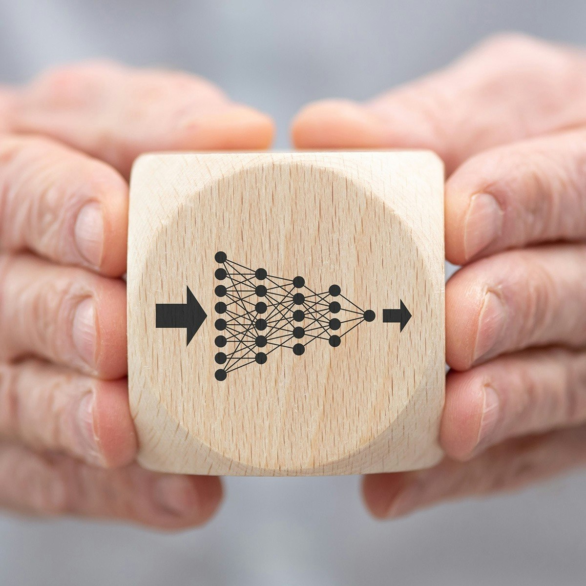


Related Reads
📰
📰
📰
📰
How to Choose the Best Deep Learning Model for Medical Imaging
Medium · Deep Learning
Another Way to Read Neural Geometry
Medium · Data Science
Another Way to Read Neural Geometry
Medium · Deep Learning
Building My First Neural Network From Scratch with PyTorch: A Journey on the Dry Bean Dataset
Medium · Deep Learning
🎓
Tutor Explanation
 DeepCamp AI